Bhisham C. Gupta - Statistics and Probability with Applications for Engineers and Scientists Using MINITAB, R and JMP

2 Enter frequencies of the categories in C2.

3 From the Menu bar select Graph Bar Chart. This prompts the following dialog box to appear on the screen:

4 Select one of the three options under Bars represent, that is, Counts of unique values, A function of variables, or Values from a table, depending upon whether the data are sample values, functions of sample values such as means of various samples, or categories and their frequencies.

5 Select one of the three possible bar charts that suits your problem. If we are dealing with only one sample from a single population, then select Simple and click OK. This prompts another dialog box, as shown below, to appear on the screen:

6 Enter C2 in the box under Graph Variables.

7 Enter C1 in the box under Categorical values.

8 There are several other options such as Chart Option, scale; click them and use them as needed. Otherwise click OK. The bar chart will appear identical to the one shown in Figure 2.4.4.

USING R

We can use built in ‘barplot()’ function in R to generate bar charts. First, we obtain the frequency table via the ‘table()’ function. The resulting tabulated categories and their frequencies are then inputted into the ‘barplot()’ function as shown in the following R code.

DefectTypes = c(2,1,3,1,2,1,5,4,3,1,2,3,4,3,1,5,2,3,1,2,3,5,4,3, 1,5,1,4,2,3,2,1,2,5,4,2,4,2,5,1,2,1,2,1,5,2,1,3,1,4) #To obtain the frequencies counts = table(DefectTypes) #To obtain the bar chart barplot(counts, xlab=‘Defect type’, ylab=‘Frequency’)

Histograms are extremely powerful graphs that are used to describe quantitative data graphically. Since the shape of a histogram is determined by the frequency distribution table of the given set of data, the first step in constructing a histogram is to create a frequency distribution table. This means that a histogram is not uniquely defined until the classes or bins are defined for a given set of data. However, a carefully constructed histogram can be very informative.

For instance, a histogram provides information about the patterns, location/center, and dispersion of the data. This information is not usually apparent from raw data. We may define a histogram as follows:

A histogram is a graphical tool consisting of bars placed side by side on a set of intervals (classes, bins, or cells) of equal width. The bars represent the frequency or relative frequency of classes. The height of each bar is proportional to the frequency or relative frequency of the corresponding class.

To construct a histogram, we take the following steps:

1 Step 1. Prepare a frequency distribution table for the given data.

2 Step 2. Use the frequency distribution table prepared in Step 1 to construct the histogram. From here, the steps involved in constructing a histogram are exactly the same as those to construct a bar chart, except that in a histogram, there is no gap between the intervals marked on the horizontal axis (the ‐axis).

A histogram is called a frequency histogram or a relative frequency histogram depending on whether the scale on the vertical axis (the ‐axis) represents the frequencies or the relative frequencies. In both types of histograms, the widths of the rectangles are equal to the class width. The two types of histograms are in fact identical except that the scales used on the ‐axes are different. This point becomes quite clear in the following example:

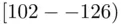
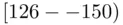
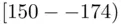
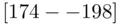
Example 2.4.5(Survival times) The following data give the survival times (in hours) of 50 parts involved in a field test under extraneous operating conditions.

60	100	130	100	115	30		145	75	80	89	57	64	92	87	110	180
195	175	179	159	155	146	157	167	174	87	67	73	109	123	135	129	141
154	166	179	37				89						39	49	190

Construct a frequency distribution table for this data. Then, construct frequency and relative frequency histograms for these data.

Solution:

1 Step 1. Find the range of the data:Then, determine the number of classes (see for example the Sturges' formula , in (2.3.2))Last, compute the class width:As we noted earlier, the class width number is always rounded up to another convenient number that is easy to work with. If the number calculated using (2.3.4) is rounded down, then some of the observations will be left out as they will not belong to any class. Consequently, the total frequency will be less than the total count of the data. The frequency distribution table for the data in this example is shown in Table 2.4.3.

2 Step 2. Having completed the frequency distribution table, construct the histograms. To construct the frequency histogram, first mark the classes on the ‐axis and the frequencies on the ‐axis. Remember that when marking the classes and identifying the bins on the ‐axis, there must be no gap between them. Then, on each class marked on the ‐axis, place a rectangle, where the height of each rectangle is proportional to the frequency of the corresponding class. The frequency histogram for the data with the frequency distribution given in Table 2.4.3is shown in Figure 2.4.5. To construct the relative frequency histogram, the scale is changed on the ‐axis (see Figure 2.4.5) so that instead of plotting the frequencies, we plot relative frequencies. The resulting graph for this example, shown in Figure 2.4.6, is called the relative frequency histogram for the data with relative frequency distribution given in Table 2.4.3.

Table 2.4.3Frequency distribution table for the survival time of parts.

		Frequency	Relative	Cumulative
Class	Tally	or count	frequency	frequency
	/////	5	5/50	5
	///// /////	10	10/50	15
	///// ////	9	9/50	24
	///// //	7	7/50	31
	///// /	6	6/50	37
	///// /	6	6/50	43
	///// //	7	7/50	50
Total		50	1

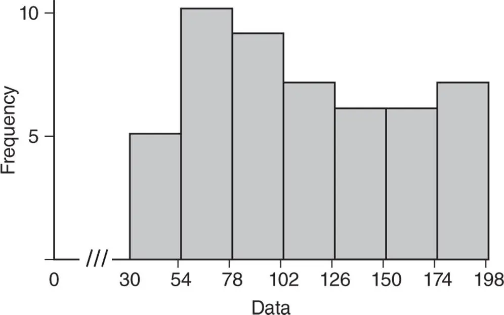
Figure 2.4.5Frequency histogram for survival time of parts under extraneous operating conditions.