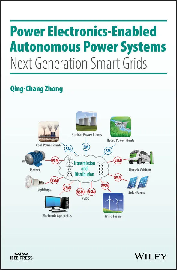
Qing-Chang Zhong - Power Electronics-Enabled Autonomous Power Systems

Figure 11.7Controller for the inverter leg.

Figure 11.8Real‐time simulation results of the transformerless PV inverter in Figure 11.5(a).

Figure 12.1STATCOM connected to a power system.

Figure 12.2A typical two‐axis control strategy for a PWM based STATCOM using a PLL.

Figure 12.3A synchronverter based STATCOM controller.

Figure 12.4Single‐line diagram of the power system used in the simulations.

Figure 12.5Detailed model of the STATCOM used in the simulations.

Figure 12.6Connecting the STATCOM to the grid.

Figure 12.7Simulation results of the STATCOM operated in different modes.

Figure 12.8Transition from inductive to capacitive reactive power when the mode was changed at t = 3.0 s from the Q ‐mode to the V ‐mode.

Figure 12.9Simulation results of the STATCOM operated with a changing grid frequency.

Figure 12.10Simulation results of the STATCOM operated with a changing grid voltage.

Figure 12.11Simulation results with a variable system strength.

Figure 13.1Per‐phase diagram with the Kron‐reduced network approach.

Figure 13.2Phase portraits of the controller.

Figure 13.3The controller to achieve bounded frequency and voltage.

Figure 13.4 E +surface (upper) and E −surface (lower) with respect to P sand Q s.

Figure 13.5Illustration of the areas characterized by E +lines and E −lines.

Figure 13.6Illustration of the area where a unique equilibrium exists.

Figure 13.7Real‐time simulation results comparing the original (SV) with the improved self‐synchronized synchronverter (improved SV).

Figure 13.8Phase portraits of the controller states in real‐time simulations.

Figure 14.1The controller of the original synchronverter.

Figure 14.2Active power regulation in a conventional synchronverter after decoupling.

Figure 14.3Properties of the active power loop of a conventional synchronverter with X pu= 0.05, ω n= 100π rad s −1, and α = 0.5%.

Figure 14.4VSM with virtual inertia and virtual damping.

Figure 14.5The small‐signal model of the active‐power loop with a virtual inertia block H v( s ).

Figure 14.6Implementations of a virtual damper.

Figure 14.7A VSM in a microgrid connected to a stiff grid.

Figure 14.8Normalized frequency response of a VSM with reconfigurable inertia and damping.

Figure 14.9Effect of the virtual damping ( J v= 0.2 s).

Figure 14.10A microgrid with two VSMs.

Figure 14.11Two VSMs operated in parallel with J v1= J v2= 1 s.

Figure 14.12Two VSMs operated in parallel with J v1= 0.5 s and J v2= 1 s.

Figure 14.13Simulation results under a ground fault with J v= 0.1, 0.3, 0.5, 1 s.

Figure 14.14Experimental results with reconfigurable inertia and damping.

Figure 14.15Experimental results from the original synchronverter for comparison.

Figure 14.16Experimental results showing the effect of the virtual damping with J v= 0.2 s.

Figure 14.17Experimental results when two VSMs with the same inertia time constant are in parallel operation.

Figure 14.18Experimental results when two VSMs with different inertia time constants operated in parallel.

Figure 14.19Experimental results when the two VSMs operated as the original SV in parallel operation with τ ω1= τ ω2= 1 s for comparison.

Figure 15.1Block diagrams of a conventional PLL.

Figure 15.2Enhanced phase‐locked loop (EPLL) or sinusoidal tracking algorithm (STA).

Figure 15.3Power delivery to a voltage source through an impedance.

Figure 15.4Conventional droop control scheme for an inductive impedance.

Figure 15.5Conventional droop control strategies.

Figure 15.6Linking the droop controller in Figure 15.4(b) and the (inductive) impedance.

Figure 15.7Droop control strategies in the form of a phase‐locked loop.

Figure 15.8The conventional droop controller shown in Figure 15.4(a) after adding two integrators and a virtual impedance.

Figure 15.9The synchronization capability of the droop controller shown in Figure 15.8.

Figure 15.10Connection of the droop controlled inverter to the grid.

Figure 15.11Regulation of the grid frequency and voltage in the droop mode.

Figure 15.12Robustness of synchronization against DC‐bus voltage changes.

Figure 15.13System response when the operation mode was changed.

Figure 16.1A single‐phase inverter.

Figure 16.2Controller to achieve a resistive output impedance.

Figure 16.3Controller to achieve a capacitive output impedance.

Figure 16.4Typical output impedances of L‐, R‐, and C‐inverters.

Figure 16.5Two R‐inverters operated in parallel.

Figure 16.6Conventional droop control scheme for R‐inverters.

Figure 16.7Experimental results: two R‐inverters in parallel with conventional droop control.

Figure 16.8Robust droop controller for R‐inverters.

Figure 16.9Experimental results for the case with a linear load when inverters have different per‐unit output impedances: with the robust droop controller (left column) and with the conventional droop controller (right column).

Figure 16.10Experimental results for the case with a linear load when inverters have the same per‐unit impedance: with the robust droop controller (left column) and with the conventional droop controller (right column).

Figure 16.11Experimental results for the case with the same per‐unit impedance using the robust droop controller: with K e= 10 (left column) and K e= 1 (right column).

Figure 16.12Experimental results with a nonlinear load: with the robust droop controller (left column) and with the conventional droop controller (right column).

Figure 16.13Robust droop controller for C‐inverters.

Figure 16.14Experimental results of C‐inverters (left column) and R‐inverters (right column) with a linear load R L= 9 Ω.

Figure 16.15Experimental results of C‐inverters (left column) and R‐inverters (right column) with a nonlinear load.

Figure 16.16Robust droop controller for L‐inverters.

Figure 16.17Experimental results of L‐inverters with a linear load: with the robust droop controller (left column) and the conventional droop controller (right column).

Figure 16.18Experimental results of L‐inverters with a nonlinear load: with the robust droop controller (left column) and with the conventional droop controller (right column).

Figure 17.1The model of a single‐phase inverter.