C. Philip Wheater - Practical Field Ecology

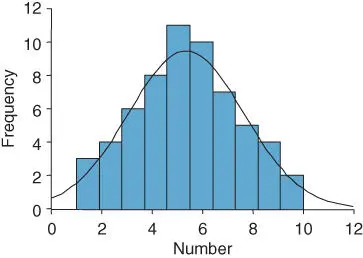
Figure 1.6 Data set approximating to a normal distribution.

We may wish to collect data to set up a model that enables us to predict the outcome in a hypothetical situation, one of the simplest of which is known as a linear regression model. Thus, if we are interested in looking at a possible relationship between woodland size and the number of birds and knew that this was likely to produce a significant linear relationship, then we may wish to use this fact to calculate the expected number of birds found in any woodland. This could be used theoretically or in conservation management to check that we have the sort of bird biodiversity that we expect from other data. Here, it is important to note that any such prediction should only be made if the woodland area in which we are interested lies between the minimum and maximum value of the data set we used to establish the model. We first need to establish which variable is the dependent and which is the independent variable: that is, which is likely to be affected (the dependent or response variable – plotted on the y axis of a scatterplot) by the other (independent variable – plotted on the x axis of a scatterplot). Here, obviously, the number of birds (the dependent variable) is more likely to be dependent on the size of the woodland (the independent variable) than vice versa. We can think of this as woodland size driving the size of the bird count. We can extend the technique to cover the case where there are a number of independent variables (e.g. woodland area, habitat diversity, area of associated green space, distance to nearest waterbody) that might influence or drive bird numbers.

Where the question to be asked is a complicated one involving a number of dependent and/or independent variables, then multivariate analyses may be appropriate. The choice of analysis depends on whether the dependent variable is a category, or a ranked or measured variable, and on whether the independent variables are categories, ranked, or measured (or even a mixture). Whilst most such analyses only have one dependent variable, there may be multiple independent variables. For example, we may want to know whether the number of birds differs in different types of woodland when we take into account the woodland size (measured variable), woodland type (nominal variable), distance to the nearest neighbouring woodland (measured variable), age of woodland (measured variable), and the land use type surrounding the woodland (nominal variable). Here, we could enter all of the data into one analysis that would take into account the interrelationships between each variable and produce a model describing the relative importance of each variable on the number of birds (this particular example could be analysed using a generalized linear model – p. 319). Such techniques are powerful but require a full understanding of the data or data set and its attributes and may be quite complex to interpret.

Ecological data sets can be very complex and difficult to visualise. For example, a data set might include many variables collected as measurements (including counts), as ranks (e.g. scores of abundance), or in a binary form (e.g. presence or absence data). Chapter 5introduces a number of techniques for visualising complex data sets to enable the use of a range of different types of data. Variables with large numbers of observations of zero (as can occur when surveying relatively rare species), cases where data are heavily skewed, or situations where variables are measured on scales of greatly differing magnitude, may require data transformation before using these techniques (p. 285).

As an example, we might collect information about woodlands on the basis of their size, age, distance to the nearest neighbouring woodland, etc. Since some of these variables will be related to each other, we might wish to find out the underlying pattern of interrelationships within the data and hence identify a number of unrelated factors that can be used instead of our large number of variables. This is a data reduction exercise, reducing the number of variables we have measured into a smaller number of unrelated factors that take into account the interrelationships between the variables.

Alternatively, we might wish to look at the range of species found in each of several woodlands and see which woodlands have similar species types. This is a similarity or clustering analysis and, depending on the technique used to calculate the similarities, data are normally recorded as a matrix (of species by woodlands) that contains either measurements (e.g. counts), ranks (e.g. ranked abundance), or binary data (e.g. species presence or absence). A similar technique to clustering enables us to visualise patterns in either the individuals (in this example, the woodlands) and/or the variables (here, the types of species). This is known as ordination and there are a number of different methods available depending on the algorithm (i.e. statistical formula). Such methods can utilise data comprising measurements, ranks, or binary information.

This chapter has identified the range of aspects that should be carefully considered when planning your project. Case Study 1.3describes how one researcher approached her work, using the current literature to develop her techniques and adopting appropriate protocols for working overseas, in potentially hazardous environments. Ensure that you take sufficient time in the planning phase of your research project to cover all of the component parts. This includes health and safety and legal issues as well as making sure that your aims and objectives are focused and that any methods employed are appropriate to gather and analyse data. At each stage, consider the details of the implementation, whether this is in the practicalities of sampling or data management. Box 1.9gives some general guidelines that should be ticked off in advance of implementing your project.

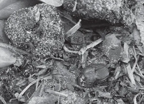Phanaeus vindex in feral hog dung.

Dr Roisin Stanbrook is a Post‐doctoral fellow at the University of Central Florida. She uses dung beetles to assess the impact of habitat modification on dung beetle communities, and models how changes in mammalian diversity in protected areas in East Africa affect dung beetle community composition. She has long held a passion for the little things that run our world, and for the need to increase awareness of insect conservation. This case study examines the different aspects of using baited pitfall trapping, which is most commonly employed method to determine dung beetle diversity, and the challenges encountered when working in protected areas in East Africa.

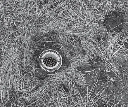A gridded pitfall trap baited with cow dung.

Scarabaeinae, or true dung beetles, comprise one of the most species‐rich groups of coprophagous insects with almost 7000 species found globally. Dung beetles have a widespread distribution, which is centred around the species‐rich tropics, with diversity gradually declining in higher latitudes. This ubiquity means that dung beetles are often used as indicators of habitat quality and barometers of habitat change due to species' associations with habitat types, and reductions in diversity when habitats are negatively affected by disturbance. One of the benefits of using dung beetles as an eco‐indicator is the ease with which large data sets can be gathered in a short timeframe, and consequentially used to form a rapid impact assessment (Bicknell et al. 2014). However, there are many challenges one may encounter when used baited pitfall traps.