Dennis M. Sullivan - Electromagnetic Simulation Using the FDTD Method with Python
Здесь есть возможность читать онлайн «Dennis M. Sullivan - Electromagnetic Simulation Using the FDTD Method with Python» — ознакомительный отрывок электронной книги совершенно бесплатно, а после прочтения отрывка купить полную версию. В некоторых случаях можно слушать аудио, скачать через торрент в формате fb2 и присутствует краткое содержание. Жанр: unrecognised, на английском языке. Описание произведения, (предисловие) а так же отзывы посетителей доступны на портале библиотеки ЛибКат.
- Название:Electromagnetic Simulation Using the FDTD Method with Python
- Автор:
- Жанр:
- Год:неизвестен
- ISBN:нет данных
- Рейтинг книги:4 / 5. Голосов: 1
-
Избранное:Добавить в избранное
- Отзывы:
-
Ваша оценка:
Electromagnetic Simulation Using the FDTD Method with Python: краткое содержание, описание и аннотация
Предлагаем к чтению аннотацию, описание, краткое содержание или предисловие (зависит от того, что написал сам автор книги «Electromagnetic Simulation Using the FDTD Method with Python»). Если вы не нашли необходимую информацию о книге — напишите в комментариях, мы постараемся отыскать её.
Electromagnetic Simulation Using the FDTD Method with Python, Third Edition Electromagnetic Simulation Using the FDTD Method with Python Guides the reader from basic programs to complex, three-dimensional programs in a tutorial fashion Includes a rewritten fifth chapter that illustrates the most interesting applications in FDTD and the advanced graphics techniques of Python Covers peripheral topics pertinent to time-domain simulation, such as Z-transforms and the discrete Fourier transform Provides Python simulation programs on an accompanying website An ideal book for senior undergraduate engineering students studying FDTD,
will also benefit scientists and engineers interested in the subject.
Electromagnetic Simulation Using the FDTD Method with Python — читать онлайн ознакомительный отрывок
Ниже представлен текст книги, разбитый по страницам. Система сохранения места последней прочитанной страницы, позволяет с удобством читать онлайн бесплатно книгу «Electromagnetic Simulation Using the FDTD Method with Python», без необходимости каждый раз заново искать на чём Вы остановились. Поставьте закладку, и сможете в любой момент перейти на страницу, на которой закончили чтение.
Интервал:
Закладка:
3 How would you write an absorbing boundary condition for a lossy material?
4 Simulate a pulse hitting a metal wall. This is very easy to do, if you remember that metal has a very high conductivity. For the complex dielectric, just use σ = 1e6 or any large number. (It does not have to be the correct conductivity of the metal, just very large.) What does this do to the FDTD parameters ca and cb? What result does this have for the field parameters Ex and Hy? If you did not want to specify dielectric parameters, how else would you simulate metal in an FDTD program?
1.A APPENDIX
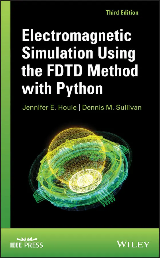
When a plane wave traveling in medium 1 strikes medium 2, the fraction that is reflected is given by the reflection coefficient Γ, and the fraction that is transmitted into medium 2 is given by the transmission coefficient τ . These are determined by the intrinsic impedances η 1and η 2of the respective media (6):
(1.A.1) 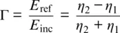
(1.A.2) 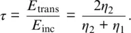
The impedances are given by
(1.A.3) 
The complex relative dielectric constant  is given by
For the case where μ = μ 0, Eq. (1.A.1)and Eq. (1.A.2)become
(1.A.4) 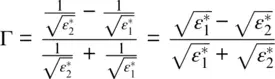
(1.A.5) 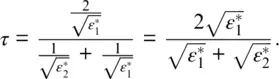
The amplitude of an electric field propagating in the positive z direction in a lossy dielectric medium is given by

where E 0is the amplitude at z = 0. The wave number k is determined by
(1.A.6) 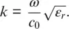
REFERENCES
1 1. K. S. Yee, Numerical solution of initial boundary value problems involving Maxwell’s equations in isotropic media, IEEE Trans. Antennas Propag., vol. 17, 1966, pp. 585–589.
2 2. A. Taflove and M. Brodwin, Numerical solution of steady state electromagnetic scattering problems using the time‐dependent Maxwell’s equations, IEEE Trans. Microwave Theory Tech., vol. 23, 1975, pp. 623–730.
3 3. A. Taflove, Computational Electrodynamics: The Finite‐Difference Time‐Domain Method, 3rd Edition, Boston, MA: Artech House, 1995.
4 4. K. S. Kunz and R. J. Luebbers, The Finite Difference Time Domain Method for Electromagnetics, Boca Raton, FL: CRC Press, 1993.
5 5. G. Mur, Absorbing boundary conditions for the finite‐difference approximation of the time domain electromagnetic field equations, IEEE Trans. Electromagn. Compat., vol. 23, 1981, pp. 377–384.
6 6. D. K. Cheng, Field and Wave Electromagnetics¸ Menlo Park, CA: Addison‐Wesley, 1992.
PYTHON PROGRAMS USED TO GENERATE FIGURES IN THIS CHAPTER
""" fd3d_1_1.py: 1D FDTD Simulation in free space """ import numpy as np from math import exp from matplotlib import pyplot as plt ke = 200 ex = np.zeros(ke) hy = np.zeros(ke) # Pulse parameters kc = int(ke / 2) t0 = 40 spread = 12 nsteps = 100 # Main FDTD Loop for time_step in range(1, nsteps + 1): # Calculate the Ex field for k in range(1, ke): ex[k] = ex[k] + 0.5 * (hy[k - 1] - hy[k]) # Put a Gaussian pulse in the middle pulse = exp(-0.5 * ((t0 - time_step) / spread) ** 2) ex[kc] = pulse # Calculate the Hy field for k in range(ke - 1): hy[k] = hy[k] + 0.5 * (ex[k] - ex[k + 1]) # Plot the outputs as shown in Fig. 1.2plt.rcParams['font.size'] = 12 plt.figure(figsize=(8, 3.5)) plt.subplot(211) plt.plot(ex, color='k', linewidth=1) plt.ylabel('E$_x$', fontsize='14') plt.xticks(np.arange(0, 201, step=20)) plt.xlim(0, 200) plt.yticks(np.arange(-1, 1.2, step=1)) plt.ylim(-1.2, 1.2) plt.text(100, 0.5, 'T = {}'.format(time_step), horizontalalignment='center') plt.subplot(212) plt.plot(hy, color='k', linewidth=1) plt.ylabel('H$_y$', fontsize='14') plt.xlabel('FDTD cells') plt.xticks(np.arange(0, 201, step=20)) plt.xlim(0, 200) plt.yticks(np.arange(-1, 1.2, step=1)) plt.ylim(-1.2, 1.2) plt.subplots_adjust(bottom=0.2, hspace=0.45) plt.show() """ fd3d_1_2.py: 1D FDTD Simulation in free space Absorbing Boundary Condition added """ import numpy as np from math import exp from matplotlib import pyplot as plt ke = 200 ex = np.zeros(ke) hy = np.zeros(ke) # Pulse parameters kc = int(ke / 2) t0 = 40 spread = 12 boundary_low = [0, 0] boundary_high = [0, 0] nsteps = 250 # Dictionary to keep track of desired points for plotting plotting_points = [ {'num_steps': 100, 'data_to_plot': None, 'label': ''}, {'num_steps': 225, 'data_to_plot': None, 'label': ''}, {'num_steps': 250, 'data_to_plot': None, 'label': 'FDTD cells'} ] # Main FDTD Loop for time_step in range(1, nsteps + 1): # Calculate the Ex field for k in range(1, ke): ex[k] = ex[k] + 0.5 * (hy[k - 1] - hy[k]) # Put a Gaussian pulse in the middle pulse = exp(-0.5 * ((t0 - time_step) / spread) ** 2) ex[kc] = pulse # Absorbing Boundary Conditions ex[0] = boundary_low.pop(0) boundary_low.append(ex[1]) ex[ke - 1] = boundary_high.pop(0) boundary_high.append(ex[ke - 2]) # Calculate the Hy field for k in range(ke - 1): hy[k] = hy[k] + 0.5 * (ex`[k] - ex[k + 1]) # Save data at certain points for later plotting for plotting_point in plotting_points: if time_step == plotting_point['num_steps']: plotting_point['data_to_plot'] = np.copy(ex) # Plot the outputs as shown in Fig. 1.3plt.rcParams['font.size'] = 12 fig = plt.figure(figsize=(8, 5.25)) def plot_e_field(data, timestep, label): """Plot of E field at a single time step""" plt.plot(data, color='k', linewidth=1) plt.ylabel('E$_x$', fontsize='14') plt.xticks(np.arange(0, 199, step=20)) plt.xlim(0, 199) plt.yticks(np.arange(0, 1.2, step=1)) plt.ylim(-0.2, 1.2) plt.text(100, 0.5, 'T = {}'.format(timestep), horizontalalignment='center') plt.xlabel('{}'.format(label)) # Plot the E field at each of the time steps saved earlier for subplot_num, plotting_point in enumerate(plotting_points): ax = fig.add_subplot(3, 1, subplot_num + 1) plot_e_field(plotting_point['data_to_plot'], plotting_point['num_steps'], plotting_point['label']) plt.tight_layout() plt.show() """ fd3d_1_3.py: 1D FDTD Simulation of a pulse hitting a dielectric medium """ import numpy as np from math import exp from matplotlib import pyplot as plt ke = 200 ex = np.zeros(ke) hy = np.zeros(ke) t0 = 40 spread = 12 boundary_low = [0, 0] boundary_high = [0, 0] # Create Dielectric Profile cb = np.ones(ke) cb = 0.5 * cb cb_start = 100 epsilon = 4 cb[cb_start:] = 0.5 / epsilon nsteps = 440 # Dictionary to keep track of desired points for plotting plotting_points = [ {'num_steps': 100, 'data_to_plot': None, 'label': ''}, {'num_steps': 220, 'data_to_plot': None, 'label': ''}, {'num_steps': 320, 'data_to_plot': None, 'label': ''}, {'num_steps': 440, 'data_to_plot': None, 'label': 'FDTD cells'} ] # Main FDTD Loop for time_step in range(1, nsteps + 1): # Calculate the Ex field for k in range(1, ke): ex[k] = ex[k] + cb[k] * (hy[k - 1] - hy[k]) # Put a Gaussian pulse at the low end pulse = exp(-0.5 * ((t0 - time_step) / spread) ** 2) ex[5] = pulse + ex[5] # Absorbing Boundary Conditions ex[0] = boundary_low.pop(0) boundary_low.append(ex[1]) ex[ke - 1] = boundary_high.pop(0) boundary_high.append(ex[ke - 2]) # Calculate the Hy field for k in range(ke - 1): hy[k] = hy[k] + 0.5 * (ex[k] - ex[k + 1]) # Save data at certain points for later plotting for plotting_point in plotting_points: if time_step == plotting_point['num_steps']: plotting_point['data_to_plot'] = np.copy(ex) # Plot the outputs as shown in Fig. 1.4plt.rcParams['font.size'] = 12 fig = plt.figure(figsize=(8, 7)) def plot_e_field(data, timestep, epsilon, cb, label): """Plot of E field at a single time step""" plt.plot(data, color='k', linewidth=1) plt.ylabel('E$_x$', fontsize='14') plt.xticks(np.arange(0, 199, step=20)) plt.xlim(0, 199) plt.yticks(np.arange(-0.5, 1.2, step=0.5)) plt.ylim(-0.5, 1.2) plt.text(70, 0.5, 'T = {}'.format(timestep), horizontalalignment='center') plt.plot((0.5 / cb - 1) / 3, 'k‐‐', linewidth=0.75) # The math on cb above is just for scaling plt.text(170, 0.5, 'Eps = {}'.format(epsilon), horizontalalignment='center') plt.xlabel('{}'.format(label)) # Plot the E field at each of the time steps saved earlier for subplot_num, plotting_point in enumerate(plotting_points): ax = fig.add_subplot(4, 1, subplot_num + 1) plot_e_field(plotting_point['data_to_plot'], plotting_point['num_steps'], epsilon, cb, plotting_point['label']) plt.subplots_adjust(bottom=0.1, hspace=0.45) plt.show() """ fd3d_1_4.py: 1D FDTD Simulation of a sinusoidal wave hitting a dielectric medium """ import numpy as np from math import pi, sin from matplotlib import pyplot as plt ke = 200 ex = np.zeros(ke) hy = np.zeros(ke) ddx = 0.01 # Cell size dt = ddx / 6e8 # Time step size freq_in = 700e6 boundary_low = [0, 0] boundary_high = [0, 0] # Create Dielectric Profile cb = np.ones(ke) cb = 0.5 * cb cb_start = 100 epsilon = 4 cb[cb_start:] = 0.5 / epsilon nsteps = 425 # Dictionary to keep track of desired points for plotting plotting_points = [ {'num_steps': 150, 'data_to_plot': None, 'label': ''}, {'num_steps': 425, 'data_to_plot': None, 'label': 'FDTD cells'} ] # Main FDTD Loop for time_step in range(1, nsteps + 1): # Calculate the Ex field for k in range(1, ke): ex[k] = ex[k] + cb[k] * (hy[k - 1] - hy[k]) # Put a sinusoidal at the low end pulse = sin(2 * pi * freq_in * dt * time_step) ex[5] = pulse + ex[5] # Absorbing Boundary Conditions ex[0] = boundary_low.pop(0) boundary_low.append(ex[1]) ex[ke - 1] = boundary_high.pop(0) boundary_high.append(ex[ke - 2]) # Calculate the Hy field for k in range(ke - 1): hy[k] = hy[k] + 0.5 * (ex[k] - ex[k + 1]) # Save data at certain points for later plotting for plotting_point in plotting_points: if time_step == plotting_point['num_steps']: plotting_point['data_to_plot'] = np.copy(ex) # Plot the outputs in Fig. 1.5plt.rcParams['font.size'] = 12 fig = plt.figure(figsize=(8, 3.5)) def plot_e_field(data, timestep, epsilon, cb, label): """Plot of E field at a single time step""" plt.plot(data, color='k', linewidth=1) plt.ylabel('E$_x$', fontsize='14') plt.xticks(np.arange(0, 199, step=20)) plt.xlim(0, 199) plt.yticks(np.arange(-1, 1.2, step=1)) plt.ylim(-1.2, 1.2) plt.text(50, 0.5, 'T = {}'.format(timestep), horizontalalignment='center') plt.plot((0.5 / cb - 1) / 3, 'k‐‐', linewidth=0.75) # The math on cb above is just for scaling plt.text(170, 0.5, 'Eps = {}'.format(epsilon), horizontalalignment='center') plt.xlabel('{}'.format(label)) # Plot the E field at each of the time steps saved earlier for subplot_num, plotting_point in enumerate(plotting_points): ax = fig.add_subplot(2, 1, subplot_num + 1) plot_e_field(plotting_point['data_to_plot'], plotting_point['num_steps'], epsilon, cb, plotting_point['label']) plt.subplots_adjust(bottom=0.2, hspace=0.45) plt.show() """ fd3d_1_5.py: 1D FDTD Simulation of a sinusoid wave hitting a lossy dielectric """ import numpy as np from math import pi, sin from matplotlib import pyplot as plt ke = 200 ex = np.zeros(ke) hy = np.zeros(ke) ddx = 0.01 # Cell size dt = ddx / 6e8 # Time step size freq_in = 700e6 boundary_low = [0, 0] boundary_high = [0, 0] # Create Dielectric Profile epsz = 8.854e-12 epsilon = 4 sigma = 0.04 ca = np.ones(ke) cb = np.ones(ke) * 0.5 cb_start = 100 eaf = dt * sigma / (2 * epsz * epsilon) ca[cb_start:] = (1 - eaf) / (1 + eaf) cb[cb_start:] = 0.5 / (epsilon * (1 + eaf)) nsteps = 500 # Main FDTD Loop for time_step in range(1, nsteps + 1): # Calculate the Ex field for k in range(1, ke): ex[k] = ca[k] * ex[k] + cb[k] * (hy[k - 1] - hy[k]) # Put a sinusoidal at the low end pulse = sin(2 * pi * freq_in * dt * time_step) ex[5] = pulse + ex[5] # Absorbing Boundary Conditions ex[0] = boundary_low.pop(0) boundary_low.append(ex[1]) ex[ke - 1] = boundary_high.pop(0) boundary_high.append(ex[ke - 2]) # Calculate the Hy field for k in range(ke - 1): hy[k] = hy[k] + 0.5 * (ex[k] - ex[k + 1]) # Plot the outputs in Fig. 1.6plt.rcParams['font.size'] = 12 plt.figure(figsize=(8, 2.25)) plt.plot(ex, color='k', linewidth=1) plt.ylabel('E$_x$', fontsize='14') plt.xticks(np.arange(0, 199, step=20)) plt.xlim(0, 199) plt.yticks(np.arange(-1, 1.2, step=1)) plt.ylim(-1.2, 1.2) plt.text(50, 0.5, 'T = {}'.format(time_step), horizontalalignment='center') plt.plot((0.5 / cb - 1) / 3, 'k‐‐', linewidth=0.75) # The math on cb is just for scaling plt.text(170, 0.5, 'Eps = {}'.format(epsilon), horizontalalignment='center') plt.text(170, -0.5, 'Cond = {}'.format(sigma), horizontalalignment='center') plt.xlabel('FDTD cells') plt.subplots_adjust(bottom=0.25, hspace=0.45) plt.show()
Читать дальшеИнтервал:
Закладка:
Похожие книги на «Electromagnetic Simulation Using the FDTD Method with Python»
Представляем Вашему вниманию похожие книги на «Electromagnetic Simulation Using the FDTD Method with Python» списком для выбора. Мы отобрали схожую по названию и смыслу литературу в надежде предоставить читателям больше вариантов отыскать новые, интересные, ещё непрочитанные произведения.


Обсуждение, отзывы о книге «Electromagnetic Simulation Using the FDTD Method with Python» и просто собственные мнения читателей. Оставьте ваши комментарии, напишите, что Вы думаете о произведении, его смысле или главных героях. Укажите что конкретно понравилось, а что нет, и почему Вы так считаете.