Dennis M. Sullivan - Electromagnetic Simulation Using the FDTD Method with Python

2 Keep increasing your incident frequency from 700 MHz upward at intervals of 300 MHz. What happens?

3 A wave packet, a sinusoidal function in a Gaussian envelope, is a type of propagating wave function that is of great interest in areas such as optics. Modify your program to simulate a wave packet.

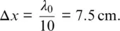
Choosing the cell size to be used in an FDTD formulation is similar to any approximation procedure: Enough sampling points must be taken to ensure that an adequate representation is made. The number of points per wavelength is dependent on many factors (3, 4). However, a good rule of thumb is 10 points per wavelength. Experience has shown this to be adequate, with inaccuracies appearing as soon as the sampling drops below this rate.

Naturally, we must use a worst‐case scenario. In general, this will involve looking at the highest frequencies we are simulating and determining the corresponding wavelength. For instance, suppose we are running simulations with 400 MHz. In free space, EM energy will propagate at the wavelength

(1.18)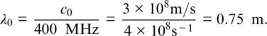

If we were only simulating free space, we would choose

However, if we are simulating EM propagation in biological tissues, for instance, we must look at the wavelength in the tissue with the highest dielectric constant, because this will have the corresponding shortest wavelength. For instance, muscle has a relative dielectric constant of about 50 at 400 MHz, so

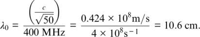
In this case, we would probably select a cell size of 1 cm.

1 Simulate a 3 GHz sine wave impinging on a material with a dielectric constant of εr = 20.

So far, we have simulated EM propagation in free space or in simple media that are specified by the relative dielectric constant ε r. However, there are many media that also have a loss term specified by the conductivity. This loss term results in the attenuation of the propagating energy.

Once more we will start with the time‐dependent Maxwell’s curl equations, but we will write them in a more general form, which allows us to simulate propagation in media that have conductivity:

(1.19a)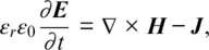

(1.19b)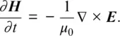

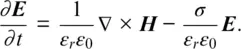
J, the current density, can also be written as

where σ is the conductivity. Putting this into Eq. (1.19a)and dividing through by the dielectric constant we get

We now revert to our simple one‐dimensional equation:

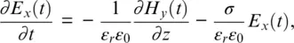
and make the change of variable in Eq. (1.5), which gives

(1.20a)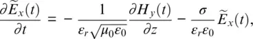

(1.20b)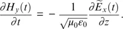

Next, take the finite‐difference approximation for both the temporal and spatial derivatives similar to Eq. (1.3a):

(1.21)

Notice that the last term in Eq. (1.20a)is approximated as the average across two time steps in Eq. (1.21). The tildes were dropped from Eq. (1.21)for simplicity. From Eq. (1.8),

so Eq. (1.21)becomes

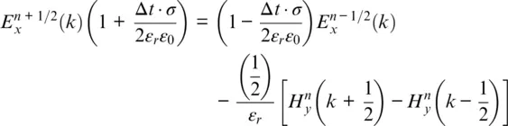
or

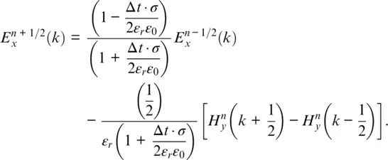
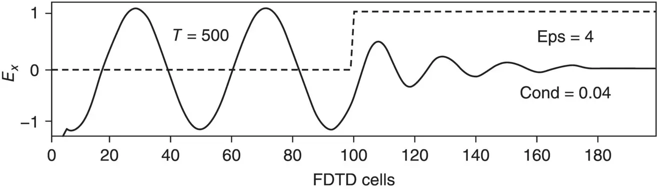
Figure 1.6 Simulation of a propagating sinusoidal wave striking a lossy dielectric material with a dielectric constant of 4 and a conductivity of 0.04 (S/m). The source is 700 MHz and originates at cell number 5.

From these we can get the computer equations:

(1.22a)

(1.22b)

where

(1.23a)

(1.23b)

(1.23c)

The program fd1d_1_5.py simulates a sinusoidal wave hitting a lossy medium that has a dielectric constant of 4 and a conductivity of 0.04. The pulse is generated at the left side and propagates to the right ( Fig. 1.6). Notice that the waveform in the medium is absorbed before it hits the boundary, so we do not have to worry about absorbing boundary conditions.

1 Run program fd1d_1_5.py to simulate a complex dielectric material. Duplicate the results of Fig. 1.6.

2 Verify that your calculation of the sine wave in the lossy dielectric is correct: That is, it is the correct amplitude going into the slab, and then it attenuates at the proper rate ( Appendix 1.A).