Dennis M. Sullivan - Electromagnetic Simulation Using the FDTD Method with Python

Suppose we are looking for a boundary condition at the end where k = 0. If a wave is going toward a boundary in free space, it is traveling at c 0, the speed of light. So, in one time step of the FDTD algorithm, it travels

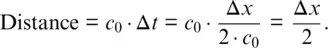
This equation shows that it takes two time steps for the field to cross one cell. A commonsense approach tells us that an acceptable boundary condition might be

(1.12)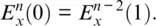

The implementation is relatively easy. Simply store a value of E x(1) for two time steps and then assign it to E x(0). Boundary conditions such as these have been implemented at both ends of the E xarray in the program fd1d_1_2.py. Figure 1.3shows the results of a simulation using fd1d_1_2.py. A pulse that originates in the center propagates outward and is absorbed without reflecting anything back into the problem space.

Figure 1.3 Simulation of an FDTD program with absorbing boundary conditions. Notice that the pulse is absorbed at the edges without reflecting anything back.

1 The program fd1d_1_2.py has absorbing boundary conditions at both ends. Get this program running and test it to ensure that the boundary conditions completely absorb the pulse.

In order to simulate a medium with a dielectric constant other than 1, which corresponds to free space, we have to add the relative dielectric constant ε rto Maxwell’s equations:

(1.13a)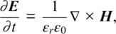

(1.13b)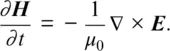

We will stay with our one‐dimensional example,

(1.14a)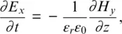

(1.14b)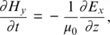

then go to the finite‐difference approximations and make the change of variables in Eq. (1.5):

(1.15a)

(1.15b)

From this we can get the computer equations

(1.16a)

(1.16b)

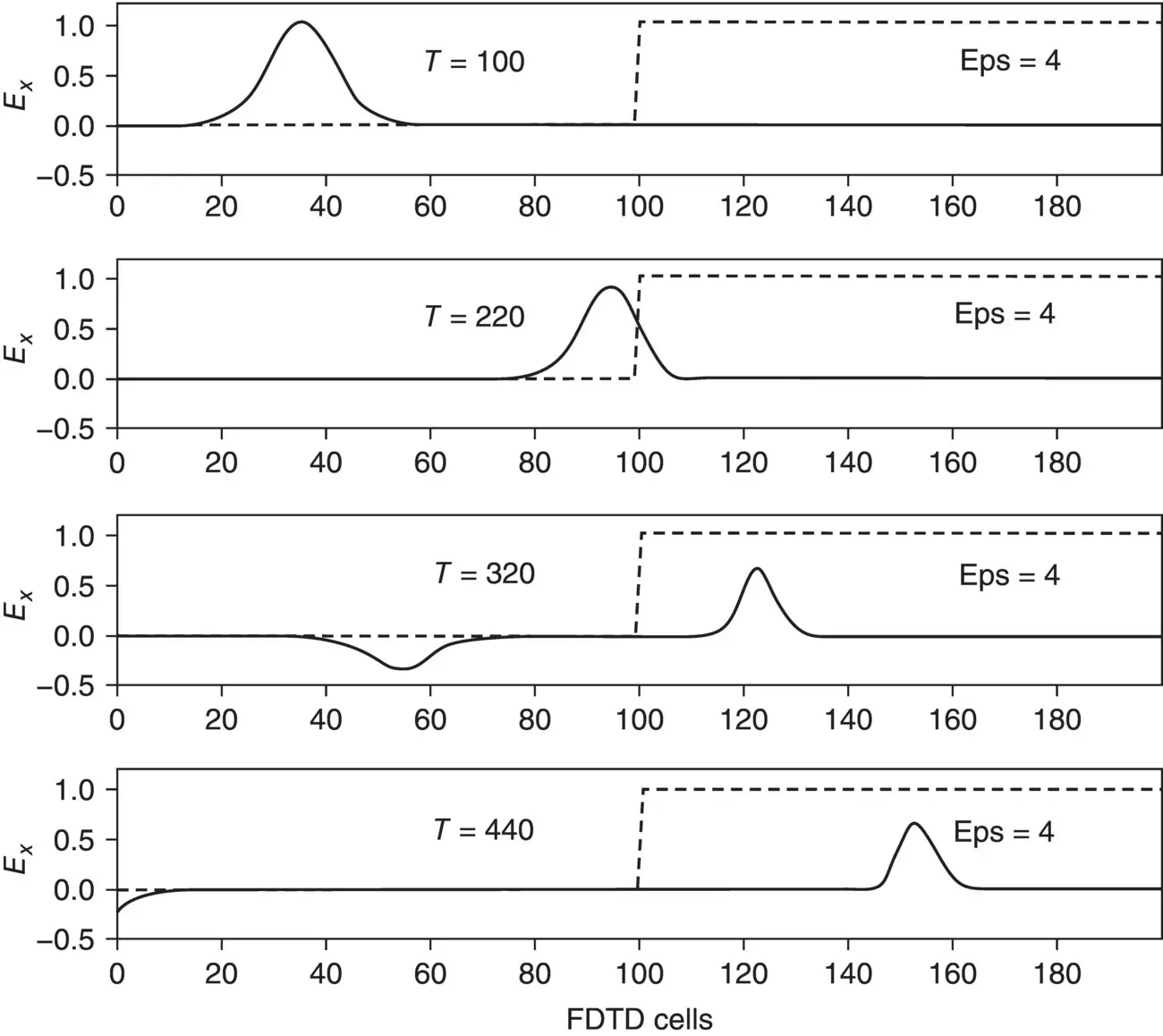
Figure 1.4 Simulation of a pulse striking dielectric material with a dielectric constant of 4. The source originates at cell number 5.

where

(1.17)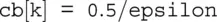

over those values of k that specify the dielectric material.

The program fd1d_1_3.py simulates the interaction of a pulse traveling in free space until it strikes a dielectric medium. The medium is specified by the parameter cbin Eq. (1.17). Figure 1.4shows the result of a simulation with a dielectric medium having a relative dielectric constant of 4. Note that one portion of the pulse propagates into the medium and the other is reflected, in keeping with basic EM theory (6).

1 The program fd1d_1_3.py simulates a problem containing partly free space and partly dielectric material. Run this program and duplicate the results of Fig. 1.4.

2 Look at the relative amplitudes of the reflected and transmitted pulses. Are they correct? Check them by calculating the reflection and transmission coefficients ( Appendix 1.A).

3 Still using a dielectric constant of 4, let the transmitted pulse propagate until it hits the far right wall. What happens? What could you do to correct this?

In the fd1d_1_1.py and fd1d_1_2.py, a source is assigned as values to E x; this is referred to as a hard source . In fd1d_1_3.py, however, a value is added to E xat a certain point; this is called a soft source . The reason is that with a hard source, a propagating pulse will see that added value and be reflected because a hard value of E xlooks like a metal wall to FDTD. With the soft source, a propagating pulse will just pass through.

Until now, we have been using a Gaussian pulse as the source. It is very easy to switch to a sinusoidal source. Just replace the parameter pulsewith the following:

The parameter freq_indetermines the frequency of the wave. This source is used in the program fd1d_1_4.py. Figure 1.5shows the same dielectric medium problem with a sinusoidal source. A frequency of 700 MHz is used. Notice that the simulation was stopped before the wave reached the far right side. Remember that we have an absorbing boundary condition, but only for free space.

Figure 1.5 Simulation of a propagating sinusoidal wave of 700 MHz striking a medium with a relative dielectric constant of 4.

In fd1d_1_4.py, the cell size ddxand the time step dtare specified explicitly. We do this because we need dtin the calculation of pulse. The cell size ddxis only specified because it is needed to calculate dtfrom Eq. (1.7).

1 Modify your program fd1d_1_3.py to simulate the sinusoidal source (see fd1d_1_4.py).