Dennis M. Sullivan - Electromagnetic Simulation Using the FDTD Method with Python

1 The Use of Normalized Units. Maxwell’s equations have been normalized by substitutingThis is a system similar to Gaussian units, which are frequently used by physicists. The reason for using it here is the simplicity in the formulation. The E and the H fields have the same order of magnitude. This has an advantage in formulating the PML, which is a crucial part of FDTD simulation.

2 Maxwell’s Equations with the Flux Density. There is some leeway in forming the time‐domain Maxwell’s equations from which the FDTD formulation is developed. The following is used in Chapter 1:(1) (2) This is a straightforward formulation and among those commonly used. However, by Chapter 2, the following formulation using the flux density is adopted:( 3) ( 4) ( 5)

In this formulation, it is assumed that the materials being simulated are nonmagnetic; that is, 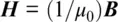. However, we will be dealing with a broad range of dielectric properties, so Eq. (4) could be a complicated convolution. There is a reason for this formulation: Eq. (3) and Eq. (5) remain the same regardless of the material; any complicated mathematics stemming from the material lies in Eq. (4). We will see that the solution of Eq. (4) can be looked upon as a digital filtering problem. In fact, the use of signal processing techniques in FDTD simulation will be a recurring theme in this book.

As mentioned above, the solution of Eq. (4) for most complicated materials can be viewed as a digital filtering problem. This being the case, the most direct approach to solve the problem is to take Eq. (4) into the Z domain. Z transforms are a regular part of electrical engineering education, but not that of physicists, mathematicians, and others. In teaching a class on FDTD simulation, Prof. Sullivan teaches some Z transform theory so when he reaches the sections on complicated dispersive materials, the students are ready to apply Z transforms. This has two distinct advantages: (a) Electrical engineering students have another application of Z transforms to strengthen their understanding of signal processing; and (b) physics students and others now know and can use Z transforms, something that had not usually been part of their formal education. Based on his positive experience, Prof. Sullivan would encourage anyone using this book when teaching an FDTD course to consider this approach. However, he has left the option open to simulate dispersive methods with other techniques. The sections on Z transforms are optional and may be skipped. Appendix Aon Z transforms is provided.

The philosophy behind this book is that the reader will learn by doing. Therefore, most exercises involve programming. Each of Chapters 1– 5has at least one FDTD program written in Python. Each of the programs is complete and can be run as written, provided the Python interpreter and necessary libraries are installed. These programs include the graphical display of results to match many of the figures in the chapters. The programs in Chapters 1– 4are designed to be simple and procedural for ease of understanding and following the equations. Chapter 5addresses some better Python programming practices and introduces some new features and techniques. This chapter attempts to introduce those unfamiliar with Python with some useful concepts to enhance FDTD programs and produce more readable, extendable code.

The programs in the book are written in Python. Python is a free, open‐source programming language which has broad adoption in both general‐purpose industries and scientific applications. This large community means that we can leverage a large number of well‐documented tools and libraries. The Python libraries are constantly being expanded. Additionally, the plotting and graphical interface libraries allow the entire program to be more interactive and user‐friendly, while being written in a high‐level language. Libraries are also available to speed up simulations to give good performance. Python, and FDTD simulations, can be run on any modern computer.

All programs in this book were run with Python 3.5.1 and the following library versions:

matplotlib==3.0.0

numba==0.39.0

numpy==1.14.3

scipy==1.0.1

This chapter provides a step‐by‐step introduction to the finite‐difference time‐domain (FDTD) method, beginning with the simplest possible problem, the simulation of a pulse propagating in free space in one dimension. This example is used to illustrate the FDTD formulation. Subsequent sections lead to formulations for more complicated media.

The time‐dependent Maxwell’s curl equations for free space are

(1.1a)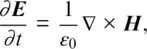

(1.1b)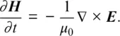

Eand Hare vectors in three dimensions, so, in general, Eq. (1.1a)and (1.1b)represent three equations each. We will start with a simple one‐dimensional case using only E xand H y, so Eq. (1.1a)and (1.1b)become

(1.2a)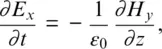

(1.2b)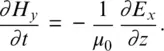

These are the equations of a plane wave traveling in the z direction with the electric field oriented in the x direction and the magnetic field oriented in the y direction.

Taking the central difference approximations for both the temporal and spatial derivatives gives

(1.3a)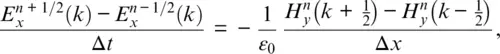

(1.3b)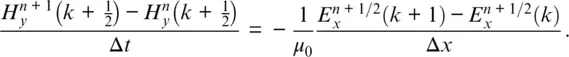

In these two equations, time is specified by the superscripts, that is, n represents a time step, and the time t is t = Δ t ⋅ n . Remember, we have to discretize everything for formulation into the computer. The term n + 1 means one time step later. The terms in parentheses represent distance, that is, k is used to calculate the distance z = Δ x ⋅ k . (It might seem more sensible to use Δ z as the incremental step because in this case we are going in the z direction. However, Δ x is so commonly used for a spatial increment that we will use Δ x .) The formulation of Eq. (1.3a)and (1.3b)assume that the E and H fields are interleaved in both space and time. H uses the arguments k + 1/2 and k − 1/2 to indicate that the H field values are assumed to be located between the E field values. This is illustrated in Fig. 1.1. Similarly, the n + 1/2 or n − 1/2 superscript indicates that it occurs slightly after or before n , respectively. Equations (1.3a)and (1.3b)can be rearranged in an iterative algorithm: