Dennis M. Sullivan - Electromagnetic Simulation Using the FDTD Method with Python

(1.4a)

(1.4b)

Notice that the calculations are interleaved in space and time. In Eq. (1.4a), for example, the new value of E xis calculated from the previous value of E xand the most recent values of H y.

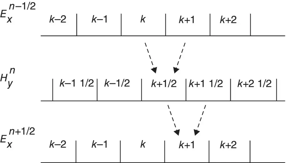
Figure 1.1 Interleaving of the E and H fields in space and time in the FDTD formulation. To calculate H y, for instance, the neighboring values of E xat k and k + 1 are needed. Similarly, to calculate E x, the values of H yat k + 1/2 and are needed.

This is the fundamental paradigm of the FDTD method (1).

Equations (1.4a)and (1.4b)are very similar, but because ε 0and μ 0differ by several orders of magnitude, E xand H ywill differ by several orders of magnitude. This is circumvented by making the following change of variables (2):

(1.5)

Substituting this into Eq. (1.4a)and (1.4b)gives

(1.6a)

(1.6b)

Once the cell size Δ x is chosen, then the time step Δ t is determined by

(1.7)

where c 0is the speed of light in free space. (The reason for this will be explained in Section 1.2.) Therefore, remembering that ε 0 μ 0= 1/( c 0) 2,

(1.8)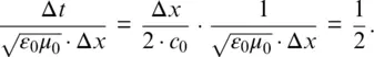

Rewriting Eq. (1.6a)and (1.6b)in Python gives the following:

(1.9a)

(1.9b)

Note that the n , n + 1/2, or n − 1/2 in the superscripts is gone. Time is implicit in the FDTD method. In Eq. (1.9a), the exon the right side of the equal sign is the previous value at n − 1/2, and the exon the left side is the new value n + 1/2, which is being calculated. Position, however, is explicit. The only difference is that k + 1/2 and k − 1/2 are rounded to k and k − 1 in order to specify a position in an array in the program.

The program fd1d_1_1.py at the end of this chapter is a simple one‐dimensional FDTD program. It generates a Gaussian pulse in the center of the problem space, and the pulse propagates away in both directions as seen in Fig. 1.2. The E xfield is positive in both directions, but the H yfield is negative in the negative direction. The following points are worth noting about the program:

1 The Ex and Hy values are calculated by separate loops, and they employ the interleaving described above.

2 After the Ex values are calculated, the source is calculated. This is done by simply specifying a value of Ex at the point k = kc and overriding what was previously calculated. This is referred to as a hard source because a specific value is imposed on the FDTD grid.

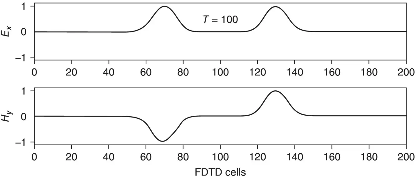
Figure 1.2 FDTD simulation of a pulse in free space after 100 time steps. The pulse originated in the center and travels outward.

1 Get the program fd1d_1_1.py running. What happens when the pulse hits the end of the array? Why?

2 Modify the program so it has two sources, one at kc ‐ 20 and one at kc + 20. (Notice that kc is the center of the problem space.) What happens when the pulses meet? Explain this from basic electromagnetic (EM) theory.

3 Instead of Ex as the source, use Hy at k = kc as the source. What difference does it make? Try a two‐point magnetic source at kc ‐ 1 and kc such that hy[kc ‐ 1] = ‐ hy[kc]. What does this look like? To what does it correspond physically?

Let us return to the discussion of how to determine the time step. An EM wave propagating in free space cannot go faster than the speed of light. To propagate a distance of one cell requires a minimum time of Δ t = Δ x / c 0. With a two‐dimensional simulation, we must allow for the propagation in the diagonal direction, which brings the requirement to . Obviously, a three‐dimensional simulation requires . This is summarized by the well‐known Courant Condition (3, 4):

(1.10)

where n is the dimension of the simulation. Unless otherwise specified, throughout this book we will determine Δ t by

(1.11)

This is not necessarily the best formula; we will use it for simplicity to avoid using square roots.

1 In fd1d_1_1.py, go to the governing equations, Eq. (1.9a)and (1.9b), and change the factor 0.5 to 1.0. What happens? Change it to 1.1. Now what happens? Change it to 0.25 and see what happens.

Absorbing boundary conditions are necessary to keep outgoing E and H fields from being reflected back into the problem space. Normally, in calculating the E field, we need to know the surrounding H values. This is a fundamental assumption of the FDTD method. At the edge of the problem space we will not have the value of one side. However, we have an advantage because we know that the fields at the edge must be propagating outward. We will use this fact to estimate the value at the end by using the value next to it (5).