George F. Elmasry - Dynamic Spectrum Access Decisions

This ROC model is the most basic model where a sensor is probing a frequency band to check for the presence or absence of a communications signal. This basic model relies on energy detection and can assume that the noise is AWGN such that the signal received by the sensor can be expressed as follows:

3.1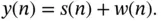

In Equation (3.1), s ( n ) is the sensed signal, w ( n ) is the AWGN, and n is the sampling index. If the sensed frequency band has no signal occupying it, then s ( n ) = 0 and the sensing process will detect the energy level of the AWGN.

The sensed signal energy can be expressed as a vector of multiple sampling points as follows:

3.2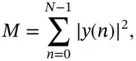

where N is the size of the observation vector.

The value of N and the definition of sampling points can differ from one sensor to another and any pre‐knowledge of the sensed signal waveform characteristics can guide the sensor into creating more optimal sampling points.

The energy detection process can compare the decision metric M from Equation (3.2)against a fixed threshold λ E. This processes needs to distinguish between two hypotheses, one hypothesis is for the presence of only noise and the other hypothesis is for the presence of signal and noise. These two hypotheses are:

3.3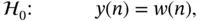

3.4

The spectrum sensor detection algorithm can successfully detect the sensed frequency with probability P Dand the noise variance can cause a false alarm 3with a probability of P F. The detection problem can be expressed as:

3.5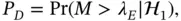

3.6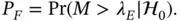

Equations (3.5)and (3.6)can be illustrated as shown in Figure 3.1where selecting an energy threshold λ Ecan deviate from the optimum threshold. The optimum threshold is not known at any given instant and would have resulted in P D= 1 and P F= 0. The estimated λ Ecan either be intentionally shifted to the right or shifted to the left as shown by the arrows at the bottom of Figure 3.1. If it is shifted to the left, the ROC model would increase the probability of hypothesizing , leading to a higher false alarm probability. If it is shifted to the right, the ROC model would increase the probability of hypothesizing , leading to a higher misdetection probability. This intentional shifting of the threshold depends on the communications system being designed. The system requirements can lead to shifting the threshold either to the left or to the right within a range, as indicated by the dashed arrow at the top of Figure 3.1.

Figure 3.1Single‐threshold ROC model leading to false alarm and misdetection.

Maximum likelihood decisions can be applied to the decision threshold λ E. A key factor in selecting λ Eis the estimation of noise power. Also, estimating the signal power by the sensor can be difficult since it can change due to propagation environments, and the distance between the transmitting node and the sensor. A good approach to select λ Eis to balance P Dand P Fbased on given requirements. The threshold λ Ecan be chosen to meet a given false alarm rate that can be deemed acceptable for the system under design. This makes it sufficient to model the noise variance, assuming a zero‐mean Gaussian random variable with variance . With this noise model, we can express the noise as 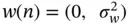. We can also simplify how we model the signal s ( n ) in order to make this analysis possible. 4We can assume that there is no fading and express the signal as a zero‐mean Gaussian variable making 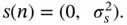5These assumptions allows us to express the decision metric M as a Chi‐square distribution with 2 N degree of freedom giving:

3.7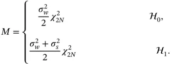

Thus, the ROC model can calculate P Dand P Fas follows:

3.8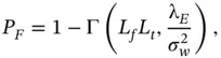

3.9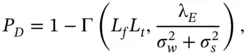

where Γ( a , x ) is the incomplete gamma function and L fand L tare the associated Laguerre polynomials.

The DSA decision fusion process can use the ROC model to compare the performances for different threshold values. ROC models are a set of convergence curves that explore the relationship between the probability of detection and the probability of a false alarm for a variety of different thresholds. Based on given requirements and machine learning techniques that count for the dynamics of the sensed environments, a close‐to‐optimal threshold can be reached. Figure 3.2exemplifies different ROC curves for different SNIR values using the equations above. SNIR is defined as the ratio of the sensed signal power to noise power .

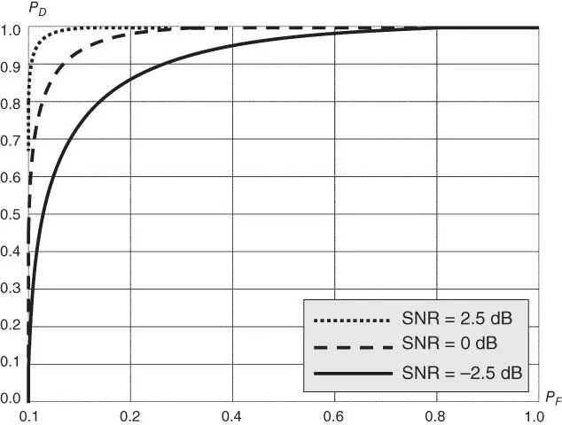
Figure 3.2Different ROC curves for different SNIR (not to scale).