George Acquaah - Principles of Plant Genetics and Breeding

The same can be done for allele a , and designated q. Further, p + q = 1 and hence p = 1 – q . If N = 80, D = 4, and H = 24,

Since p + q = 1, q = 1 − p , and hence q = 1 – 0.2 = 0.8.

Consider a random mating population (each male gamete has an equal chance of mating with any female gamete). Random mating involving the previous locus (A/a) will yield the following genotypes: AA, Aa, and aa , with the corresponding frequencies of p 2 , 2pq, and q 2, respectively. The gene frequencies must add up to unity. Consequently, p 2 + 2pq + q 2= 1. This mathematical relationship is called the Hardy‐Weinberg equilibrium. Hardy of England and Weinberg of Germany discovered that equilibrium between genes and genotypes is achieved in large populations. They showed that the frequency of genotypes in a population depends on the frequency of genes in the preceding generation, not on the frequency of the genotypes.

Considering the previous example, the genotypic frequencies for the next generation following random mating can be calculated as follows:

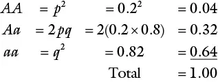
The Hardy‐Weinberg equilibrium is hence summarized as:

This means that in a population of 80 plants as before, about 3 plants will have a genotype of AA , 26 will be Aa , and 51, aa . Using the previous formula, the frequencies of the genes in the next generation may be calculated as:

and q = 1 – p = 0.8.

The allele frequencies have remained unchanged, while the genotypic frequencies have changed from 4, 24, and 52, to 3, 26, and 51, for AA, Aa, and aa , respectively. However, in subsequent generations, both the genotype and gene frequencies will remain unchanged, provided:

1 Random mating occurs in a very large diploid population.

2 Allele A and allele a are equally fit (one does not confer a superior trait than the other).

3 There is no differential migration of one allele into or out of the population.

4 The mutation rate of allele A is equal to that of allele a.

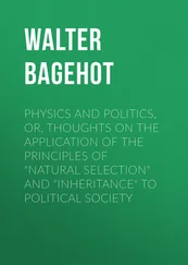
In other words, the variability does not change from one generation to another in a random mating population. The maximum frequency of the heterozygote (H) cannot exceed 0.5 ( Figure 3.1). The Hardy‐Weinberg law states that equilibrium is established at any locus after one generation of random mating. From the standpoint of plant breeding, two states of variability are present: two homozygotes ( AA, aa ), called “free variability” that can be fixed by selection; and the intermediate heterozygous ( Aa ), called “hidden or potential variability” that can generate new variability through segregation. In outcrossing species, the homozygotes can hybridize to generate more heterozygotic variability. Under random mating and no selection, the rate of crossing and segregation will be balanced to maintain the proportion of free and potential variability at 50% : 50%. In other words, the population structure is maintained as a dynamic flow of crossing and segregation. However, with two loci under consideration, equilibrium will be attained slowly over many generations. If genetic linkage is strong, the rate of attainment of equilibrium will even be much slower.

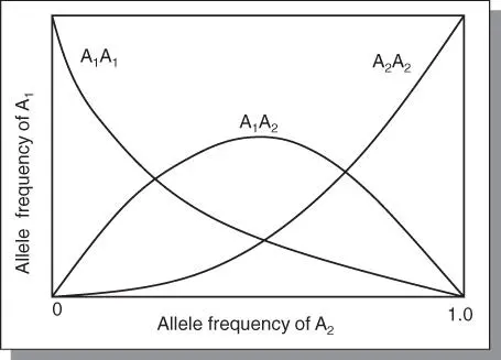
Figure 3.1The relationship between gene frequencies and allele frequencies in a population in Hardy‐Weinberg equilibrium for two alleles is depicted in the figure. The frequency of the heterozygotes cannot be more than 50%, and this maximum occurs when the gene frequencies are p = q = 0.5. Further, when the frequency of an allele is low, the rare allele occurs predominantly in heterozygotes and there are very few homozygotes.

Source: Adapted from Falconer (1981).

Most of the important variation displayed by nearly all plant characters affecting growth, development, and reproduction is quantitative (continuous or polygenic variation; controlled by many genes). Polygenes demonstrate the same properties in terms of dominance, epistasis, and linkage as classical Mendelian genes. The Hardy‐Weinberg equilibrium is applicable to these characters. However, it is more complex to demonstrate.

Another state of variability is observed when more than one gene affects the same polygenic trait. Consider two independent loci with two alleles each: A, a and B, b . Assume also the absence of dominance or epistasis. It can be shown that nine genotypes ( AABB, AABb, AaBb, Aabb, AaBB, AAbb, aaBb, aaBB, aabb ) and five phenotypes ( [AABB, 2AaBB] + [2AABb; AAbb, aaBB] + [4AaBb, 2aaBb] + [2Aabb] + [aabb]) in a frequency of 1 : 4 : 6 : 4 : 1, will be produced, following random mating. Again, the extreme genotypes ( AABB, aabb ) are the source of completely free variability. But, also AAbb and aaBB , phenotypically similar but contrasting genotypes, contain latent variability. Termed homozygotic potential variability, it will be expressed in free state only when, through crossing, a heterozyote ( AaBb ) is produced, followed by segregation in the F 2. In other words, two generations will be required to release this potential variability in free state. Further, unlike the 50% : 50% ratio in the single locus example, only 1/8 of the variability is available for selection in the free state, the remainder existing as hidden in the heterozygotic or homozygotic potential states. A general mathematical relationship may be derived for any number (n) of genes as 1 : n : n − 1 of free:heterozygotic potential:homozygotic potential.

Another level of complexity may be factored in by considering dominance and non‐allelic interactions ( AA = Aa = BB = Bb ). If this is so, the nine genotypes previously observed will produce only three phenotypic classes ( [AABB, 4AaBb, 2AaBB, 2AABb] + [2Aabb, 2aaBb, AAbb, aaBB] + [aabb ]), in a frequency of 9 : 6 : 1. A key difference is that 50% of the visible variability is now in the heterozygous potential state that cannot be fixed by selection. The heterozygotes now contribute to the visible instead of the cryptic variability. From the plant breeding standpoint, its effect is to reduce the rate of response to phenotypic selection at least in the same direction as the dominance effect. This is because the fixable homozygotes are indistinguishable from the heterozygotes without a further breeding test (e.g. progeny row). Also, the classifications are skewed (9 : 6 : 1) in the positive (or negative) direction.

A key plant breeding information to be gained from the above discussion is that in outbreeding populations, polygenic systems are capable of storing large amounts of cryptic variability. This can be gradually released for selection to act on through crossing, segregation, and recombination. The flow of this cryptic variability to the free state depends on the rate of recombination (which also depends on the linkage of genes on the chromosomes and the breeding system).