Philippe J. S. De Brouwer - The Big R-Book

file.choose()

or by providing the file name directly:

t <- readLines(“R.book.txt”)

readLines()

This will load the text of the file in one character string t. However, typically that is not exactly what we need. In order to manipulate data and numbers, it will be necessary to load data in a vector or data-frame for example.

In further sections – such as Chapter 15“ Connecting R to an SQL Database ” on page 327 – we will provide more details about data-input. Below, we provide a short overview that certainly will come in handy.

For the example we have first downloaded the CSV file with currency exchange rates from http://www.ecb.europa.eu/stats/policy_and_exchange_rates/euro_reference:exchange_rates/html/index.en.html. 4 This file is now on a local hard-drive and will be read in from there. 5

CSV

import – csv

# To read a CSV-file it needs to be in the current directory # or we need to supply the full path. getwd() # show actual working directory setwd(“./data”) # change working directorydata <- read.csv(“eurofxref-hist.csv”) is.data.frame(data) ncol(data) nrow(data) head(data) hist(data $CAD, col = ‘khaki3’) plot(data $USD, data $CAD, col = ‘red’)

In the aforementioned example, we have first copied the file to our local computer, but that is not necessary. The function read.csv()is able to read a file directly from the Internet.

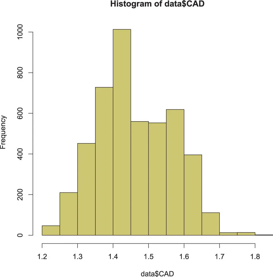
Figure 4.4 : The histogram of the CAD.

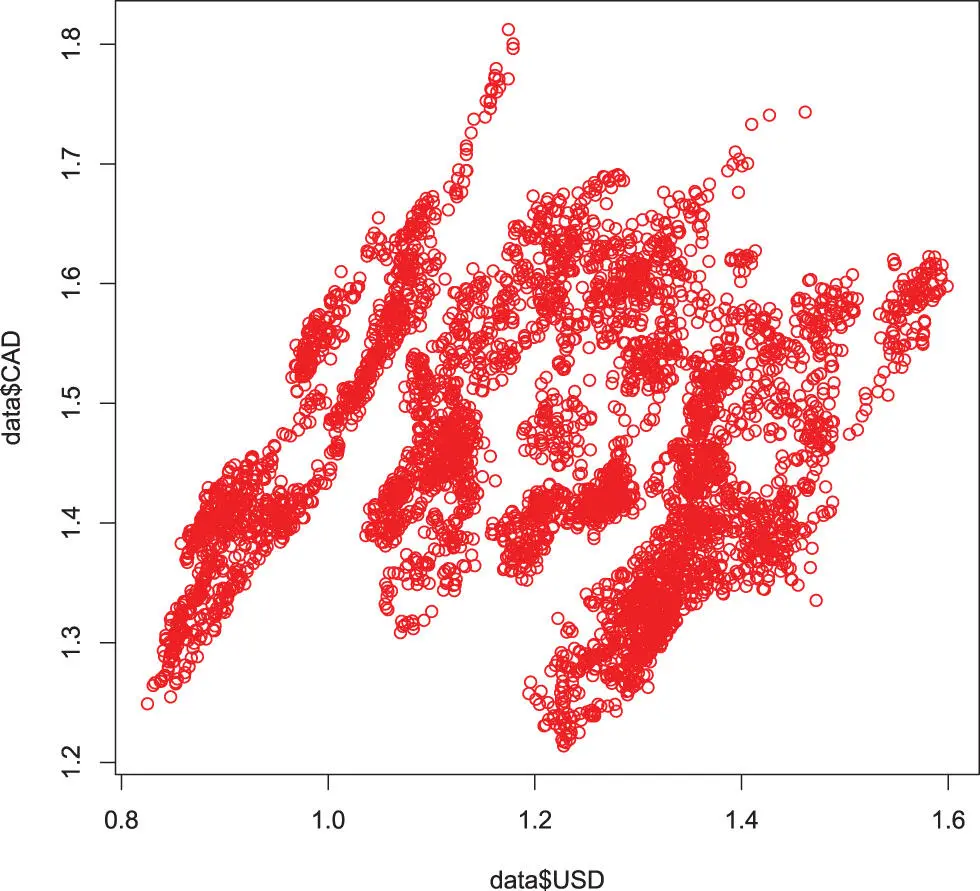
Figure 4.5 : A scatter-plot of one variable with another.

Once the data is loaded in R it is important to be able to make selections and further prepare the data.We will come back to this in much more detail in Part IV “ DataWrangling ” on page 335, but present here already some essentials.

# get the maximum exchange ratemaxCAD <- max(data $CAD) # use SQL-like selectiond0 <- subset(data, CAD ==maxCAD) d1 <- subset(data, CAD >maxCAD -0.1) d1[,1] ## [1] 2008-12-30 2008-12-29 2008-12-18 1999-02-03 ## [5] 1999-01-29 1999-01-28 1999-01-27 1999-01-26 ## [9] 1999-01-25 1999-01-22 1999-01-21 1999-01-20 ## [13] 1999-01-19 1999-01-18 1999-01-15 1999-01-14 ## [17] 1999-01-13 1999-01-12 1999-01-11 1999-01-08 ## [21] 1999-01-07 1999-01-06 1999-01-05 1999-01-04 ## 4718 Levels: 1999-01-04 1999-01-05 … 2017-06-05 d2 <- data.frame(d1 $Date,d1 $CAD) d2 ## d1.Date d1.CAD ## 1 2008-12-30 1.7331 ## 2 2008-12-29 1.7408 ## 3 2008-12-18 1.7433 ## 4 1999-02-03 1.7151 ## 5 1999-01-29 1.7260 ## 6 1999-01-28 1.7374 ## 7 1999-01-27 1.7526 ## 8 1999-01-26 1.7609 ## 9 1999-01-25 1.7620 ## 10 1999-01-22 1.7515 ## 11 1999-01-21 1.7529 ## 12 1999-01-20 1.7626 ## 13 1999-01-19 1.7739 ## 14 1999-01-18 1.7717 ## 15 1999-01-15 1.7797 ## 16 1999-01-14 1.7707 ## 17 1999-01-13 1.8123 ## 18 1999-01-12 1.7392 ## 19 1999-01-11 1.7463 ## 20 1999-01-08 1.7643 ## 21 1999-01-07 1.7602 ## 22 1999-01-06 1.7711 ## 23 1999-01-05 1.7965 ## 24 1999-01-04 1.8004 hist(d2 $d1.CAD, col = ‘khaki3’)

It is also possible to write data back into a file. Best is to use a structured format such as a CSV-file.

subset()

write.csv(d2, “output.csv”, row.names = FALSE) new.d2 <- read.csv(“output.csv”) print(new.d2) ## d1.Date d1.CAD ## 1 2008-12-30 1.7331 ## 2 2008-12-29 1.7408 ## 3 2008-12-18 1.7433 ## 4 1999-02-03 1.7151 ## 5 1999-01-29 1.7260 ## 6 1999-01-28 1.7374 ## 7 1999-01-27 1.7526 ## 8 1999-01-26 1.7609 ## 9 1999-01-25 1.7620 ## 10 1999-01-22 1.7515 ## 11 1999-01-21 1.7529 ## 12 1999-01-20 1.7626 ## 13 1999-01-19 1.7739 ## 14 1999-01-18 1.7717 ## 15 1999-01-15 1.7797 ## 16 1999-01-14 1.7707 ## 17 1999-01-13 1.8123 ## 18 1999-01-12 1.7392 ## 19 1999-01-11 1.7463 ## 20 1999-01-08 1.7643 ## 21 1999-01-07 1.7602 ## 22 1999-01-06 1.7711 ## 23 1999-01-05 1.7965 ## 24 1999-01-04 1.8004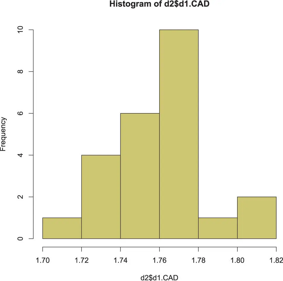

Figure 4.6 : The histogram of the most recent values of the CAD only.

Without the row.names = FALSEstatement, the function write.csv()would add a row that will get the name “X.”

Microsoft's Excel is omnipresent in the corporate environment and many people will have some data in that format. There is no need to to first save the data as a CSV file and then upload in R. The package xlsxwill allow us to directly import a file in xlsx format.

Excel

.xlx

Importing and xlsx-file is very similar to importing a CSV-file.

# install the package xlsx if not yet done if( !any( grepl(“xlsx”, installed.packages()))){ install.packages(“xlsx”)} library(xlsx) data <- read.xlsx(“input.xlsx”, sheetIndex = 1)

Spreadsheets and CSV-file are good carriers for reasonably small datasets. Any company that holds a lot of data will use a database system – see for example Chapter 13“ RDBMS ” on page 285. Importing data from a database system is somewhat different. The data is usually structured in “tables” (logical units of rectangular data); however, they will seldom contain all information that we need and usually have too much rows.We need also some protocol to communicate with the database: that is the role of the structured query language (SQL) – see Chapter 14“ SQL on page 291.

database – MySQL

R can connect to many popular database systems. For example, MySQL: as usual there is a package that will provide this functionality.

MySQL

if( !any( grepl(“xls”, installed.packages()))){ install.packages(“RMySQL”)} library(RMySQL)

RMySQL

This is explained in more detail in Chapter 15“ Connecting R to an SQL Database ” on page 327, but the code segment below will already get you the essential ingredients.