Michael Begon - Ecology

microclimatic variation

On a smaller scale still there can be a great deal of microclimatic variation. For example, the sinking of dense, cold air into the bottom of a valley at night can make it as much as 30°C colder than the side of the valley only 100 m higher; the winter sun, shining on a cold day, can heat the south‐facing side of a tree (and the habitable cracks and crevices within it) to as high as 30°C; and the air temperature in a patch of vegetation can vary by 10°C over a vertical distance of 2.6 m from the soil surface to the top of the canopy. Hence, we need not confine our attention to global or geographic patterns when seeking evidence for the influence of temperature on the distribution and abundance of organisms.

ENSO and NAO

Long‐term temporal variations in temperature, such as those associated with the ice ages, were discussed in the previous chapter ( Section 1.4.3). Between these, however, and the very obvious daily and seasonal changes that we are all aware of, a number of medium‐term patterns have become increasingly apparent. Notable amongst these are the El Niño–Southern Oscillation (ENSO) and the North Atlantic Oscillation (NAO). The ENSO is an alternation between a warm (El Niño) and a cold (La Niña) state of the waters of the tropical Pacific Ocean off the coast of South America ( Figure 2.16a), although it affects temperature and the climate generally in terrestrial and marine environments throughout the whole Pacific basin and beyond ( Figure 2.16b). The NAO refers to a north–south alternation in atmospheric mass between the subtropical Atlantic and the Arctic ( Figure 2.16c) and again affects climate in general rather than just temperature ( Figure 2.16d). Positive index values ( Figure 2.16c) are associated, for example, with relatively warm conditions in North America and Europe and relatively cool conditions in North Africa and the Middle East. An example of the effect of NAO variation on species abundance, that of cod, Gadus morhua , in the Barents Sea, is shown in Figure 2.17.

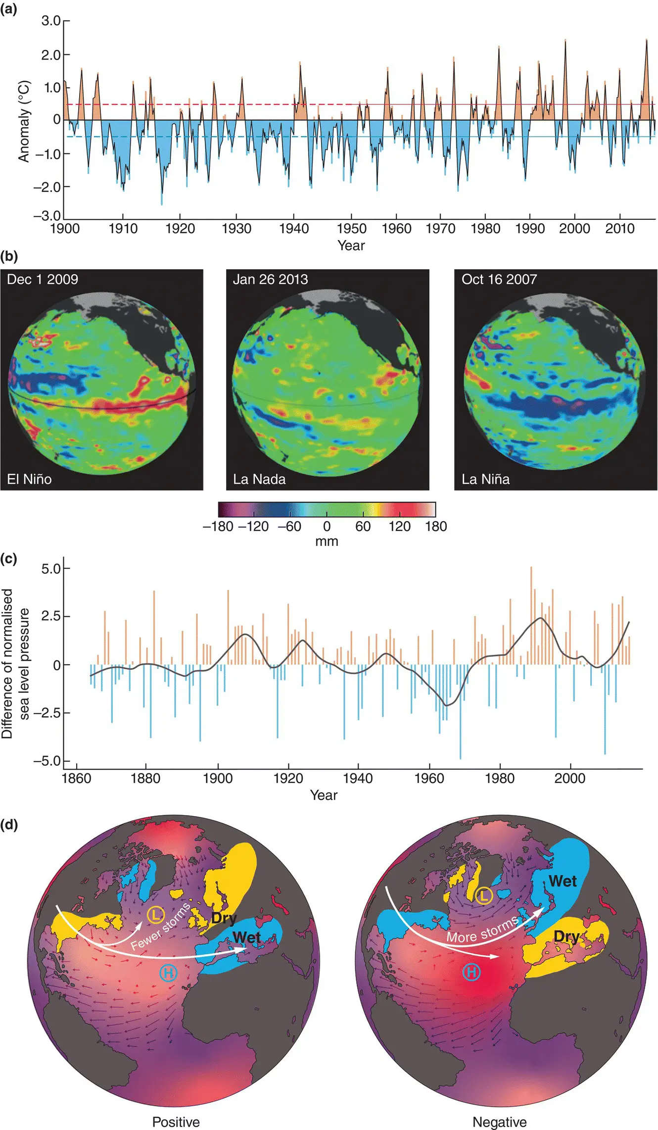
Figure 2.16 Features of the El Niño–Southern Oscillation (ENSO) and the North Atlantic Oscillation (NAO).(a) ENSO from 1900 to 2017 as measured by sea surface temperature (SST) anomalies (differences from the mean) in the equatorial mid‐Pacific. El Niño events are defined as occurring when the SST is more than 0.4°C above the mean (red dashed line) and La Niña events when the SST is more than 0.4°C below the mean (blue dashed line). (b) Examples of El Niño (December 2009) and La Niña events (October 2007) as well as a neutral state (La Nada; January 2013) in terms of sea height above average levels. Warmer seas are higher; for example, a sea height 150–200 mm below average equates to a temperature anomaly of approximately 2–3°C. (c) NAO from 1864 to 2017 as measured by the normalised sea‐level pressure difference between Lisbon in Portugal and Reykjavik in Iceland. (d) Typical winter conditions when the NAO index is positive or negative. Conditions that are more than usually warm, cold, dry or wet are indicated. The positions of the Icelandic low pressure (L) and the Azores high pressure (H) zones are shown.

Source : (a) Compiled from the US National Ocean and Atmospheric Administration (NOAA), https://www.ncdc.noaa.gov/teleconnections/enso/indicators/sst.php). (b) From the US National Aeronautics and Space Administration (NASA), https://sealevel.jpl.nasa.gov/science/elninopdo/elnino/). (c) From https://climatedataguide.ucar.edu/climate‐data/hurrell‐north‐atlantic‐oscillation‐nao‐index‐station‐based). (d) From http://www.ldeo.columbia.edu/NAO/.

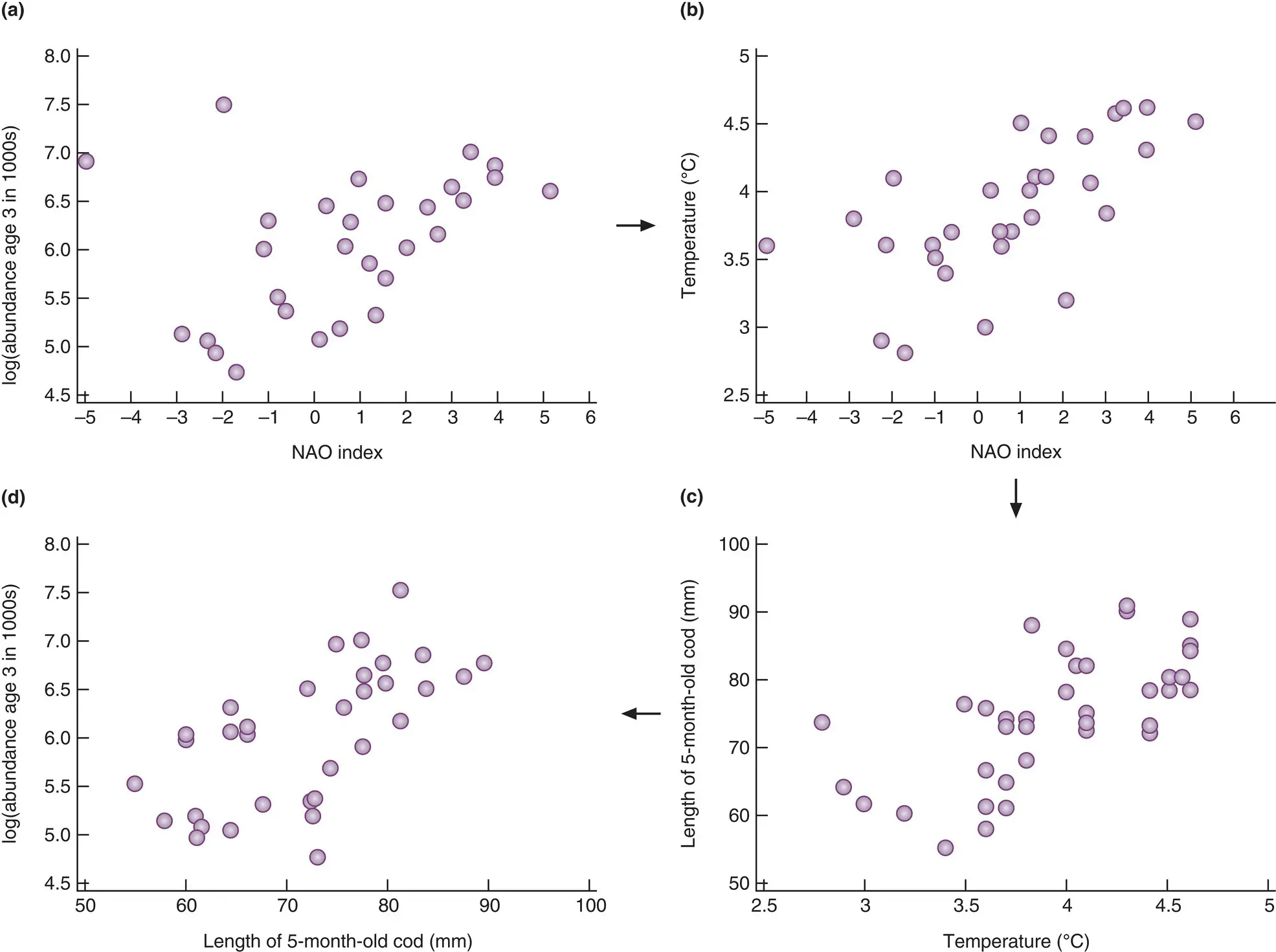
Figure 2.17 The abundance of three‐year‐old cod, Gadus morhua, in the Barents Sea is positively correlated with the value of the North Atlantic Oscillation (NAO) index.The mechanism underlying the correlation (a) is suggested in (b–d). (b) Annual mean temperature increases with the NAO index. (c) The length of five‐month‐old cod increases with annual mean temperature. (d) The abundance of cod at age three years increases with their length at five months.

Source : After Ottersen et al . (2001).

isotherms

There are very many examples of plant and animal distributions that are strikingly correlated with some aspect of environmental temperature (e.g. Figure 2.2a) and this kind of pattern may still hold even at gross taxonomic and systematic levels ( Figure 2.18). At a finer scale, the distributions of many species closely match maps of some aspect of temperature. For example, the northern cool range boundary of wild madder plants ( Rubia peregrina ) is closely correlated with the position of the January 4.5°C isotherm (an isotherm is a line on a map joining places that experience the same temperature).

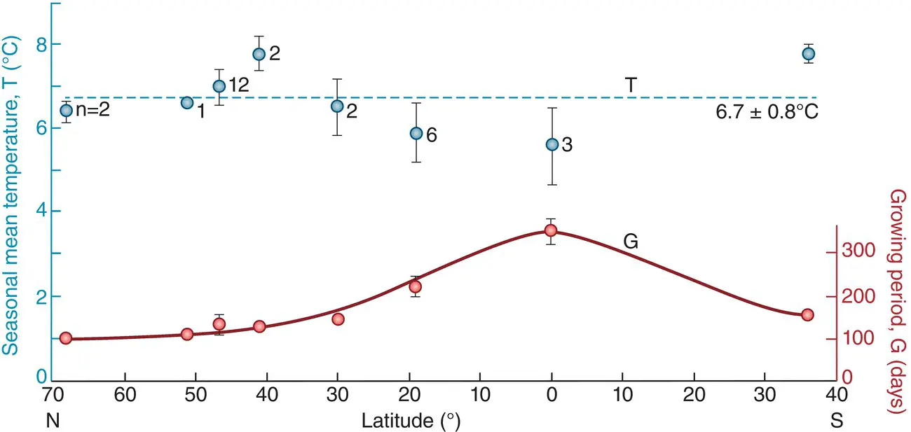
Figure 2.18 The treelines (high‐altitude limits of forest cover) of the world’s mountains seem to follow a common isotherm.This is 6.7 ± 0.8ºC), with very similar mean ground temperatures during the growing season across a wide range of latitudes from subarctic through equatorial areas to temperate southern hemisphere regions (the growing period differs according to latitude). The species composition of the forests is, of course, vastly different in the different regions.

Source : From Körner & Paulsen (2004).

However, such relationships need to be interpreted with some caution: they can be extremely valuable in predicting where we might and might not find a particular species (e.g. Figure 2.5); they may suggest that some feature related to temperature is important in the life of the organisms; but they do not prove that temperature causes the limits to a species’ distribution. For one thing, the temperatures measured for constructing isotherms for a map are only rarely those that the organisms experience. In nature an organism may choose to lie in the sun or hide in the shade and, even in a single day, may experience a baking midday sun and a freezing night. Moreover, temperature varies from place to place on a far finer scale than will usually concern a geographer, but it is the conditions in these ‘microclimates’ that will be crucial in determining what is habitable for a particular species. For example, the prostrate shrub Dryas octopetala is restricted to altitudes exceeding 650 m in north Wales, UK, where it is close to its southern limit. But to the north, in Sutherland in Scotland, where it is generally colder, it is found right down to sea level.

On the other hand, Payne et al . (2016) were able to demonstrate a strong correlation between the warm boundary isotherms of nine well‐studied fish species and their optimum temperatures for activity, somatic growth and reproductive growth ( Figure 2.19): this is good evidence of a causal link.

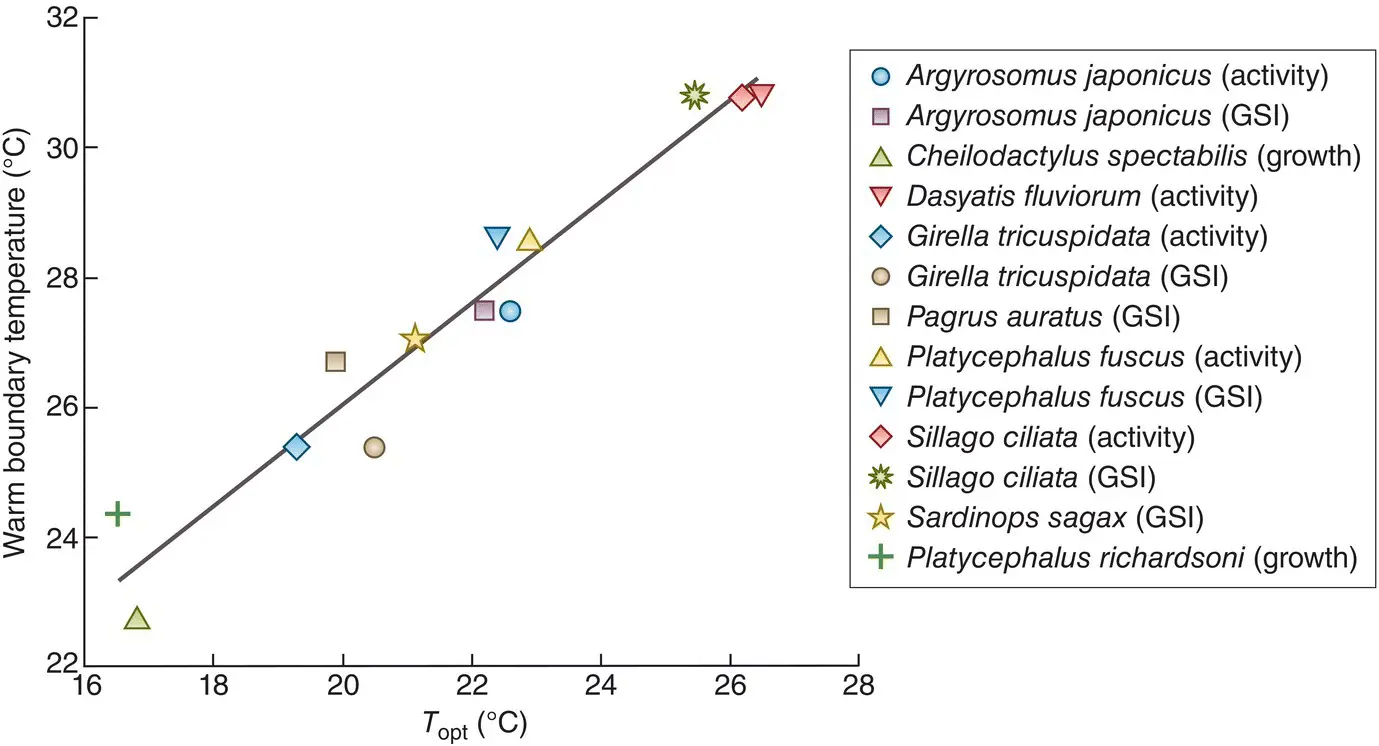
Figure 2.19 Warm boundary limits of nine Australian fish species are correlated with species‐specific optimum fish performance.Optimum temperature ( T opt) is shown for maximum activity, somatic growth or reproductive growth (gonadosomatic index, GSI, a measure of gonad mass relative to total body mass) measured in the wild (four species provided both activity and reproductive growth data, giving 13 points in total). The species‐specific warm equatorward range boundary is the average temperature of the warmest month at the range limit.