David Machin - Medical Statistics

Diagnostics tests use patient data to classify individuals as either normal or abnormal. A related statistical problem is the description of the variability in normal individuals, to provide a basis for assessing the test results of other individuals. The most common form of presenting such data is as a range of values or interval that contains the values obtained from the majority of a sample of normal subjects. The reference interval is often referred to as a normal range or reference range. To distinguish the use of the same word for the Normal distribution we have used a lower case, for the normal range, and upper case convention throughout this book.

We can use the fact that our sample birthweight data, from the O'Cathain et al. (2002) study (see Figure 4.9); appear Normally distributed to calculate a reference range for birthweights. We have already mentioned that about 95% of the observations from a Normal distribution lie within 1.96 SDs either side of the mean. So a reference range obtained from this sample of babies is:

If the baby data were not Normally distributed then the normal reference range is obtained from the calculated percentiles of the sample as described in Chapter 2. Thus the 2.5 percentile corresponds to 2.5% of the babies below this weight which equals 2.91 kg. Correspondingly the estimated 97.5 percentile suggests that only 2.5% of babies are heavier than 4.43 kg at birth. The percentile‐based reference range for baby birthweight is therefore estimated to be 2.19 to 4.43 kg. This is very close to that obtained when we assume the birthweight has a Normal distribution.

Most reference ranges are based on samples larger than 3500 people. Over many years, and millions of births, the World Health Organization (WHO) has come up with a normal birthweight range for new‐born babies. These ranges represent results than are acceptable in new‐born babies and actually cover the middle 80% of the population distribution, that is, the 10th and 90th centiles. Low birthweight babies are usually defined (by the WHO) as weighing less than 2500 g (the 10th centile) regardless of gestational age, and large birth weight babies are defined as weighing above 4000 g (the 90th centile). Hence the normal birth weight range is around 2.5 to 4.0 kg. For our sample data, the 10th to 90th centile range was similar, at 2.75 to 4.03 kg.

There are many other probability distributions used in statistics. In this section we briefly list and describe those that are more commonly used.

Student's t‐ distribution is any member of a family of continuous probability distributions that arises when estimating the mean of a Normally distributed variable (in the population) in situations where the sample size is small and the population standard deviation is unknown. It was developed by William Sealy Gosset under the pseudonym Student.

The t ‐distribution plays an important role in a number of widely used statistical analyses, including Student's t ‐test for assessing the statistical significance of the difference between two sample means, the construction of confidence intervals for the difference between two population means, and in linear regression analysis.

The t ‐distribution is symmetric and bell‐shaped, like the Normal distribution, but has heavier tails, meaning that it is more prone than a Standard Normal distribution to producing values that fall far from its mean ( Figure 4.14a). The exact shape of the t ‐distribution is determined by the mean and variance plus what are known as the degrees of freedom, df . These are derived from the sample size. As the df increases, the shape of the t ‐distribution becomes closer to the Normal distribution; and when the sample size (and degrees of freedom) are greater than 30, the t ‐distribution is very similar to the Standard Normal distribution.

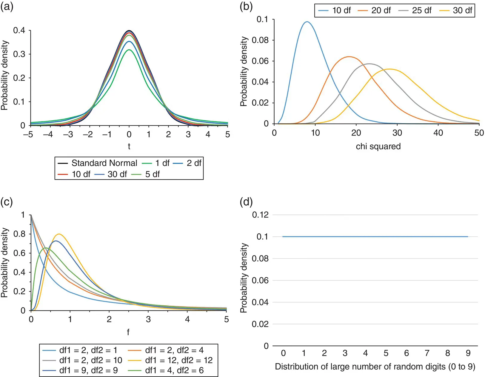
Figure 4.14 Examples of probability density/distribution functions for the t‐, chi‐squared, F‐ and Uniform distributions. (a) t ‐distribution. (b) chi‐squared distribution. (c) F ‐distribution. (d) Uniform distribution.

The chi‐squared distribution (or χ 2‐distribution) with n degrees of freedom ( Figure 4.14b) is the distribution of a sum of the squares of n independent standard Normal random variables. The chi‐squared distribution is always positive and its shape is uniquely determined by the degrees of freedom. The distribution becomes more symmetrical as the degrees of freedom increase and when the degrees of freedom are greater than 50, the chi‐squared distribution is very similar to the Normal distribution. The chi‐squared distribution is used in the common chi‐squared tests for goodness of fit of an observed distribution to a theoretical one, the independence of two criteria of classification of qualitative data, and in confidence interval estimation for a population standard deviation of a Normal distribution from a sample standard deviation.

The F ‐distribution ( Figure 4.14c) is the distribution of the ratio of two chi‐squared distributions and is used in hypothesis testing when we want to compare variances, such as in one‐way analysis of variance (see Section 7.3). It is always positive, but the exact shape depends on the degrees of freedom for the two chi‐squared distributions that determine it.

The Uniform distribution ( Figure 4.14d) has a rectangular shape so that each possible value occurs with equal probability within a given range. It can be useful in a Bayesian analysis as the prior distribution of an unknown parameter where all values with a given range are thought to be equally likely.

1 What is the population from which the sample was taken? Are there any possible sources of bias that may affect the estimates of the population parameters?

2 Have reference ranges been calculated on a random sample of healthy volunteers? If not, how does this affect your interpretation? Is there any good reason why a random sample was not taken?

3 For any continuous variable, are the variables correctly assumed to have a Normal distribution? If not, how do the investigators take account of this?

Data that can take only a 0 or 1 response, such as treatment failure or treatment success, follow the Binomial distribution provided the underlying population response rate π does not change. The Binomial probabilities are calculated from

(4.1)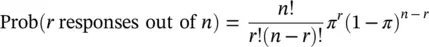

for successive values of r from 0 through to n . In the above n ! is read as n factorial and r ! as r factorial. For r = 4, r ! = 4 × 3 × 2 × 1 = 24. Both 0! and 1! are taken as equal to unity. It should be noted that the expected value for r , the number of successes yet to be observed if we treated n patients, is nπ . The potential variation about this expectation is expressed by the corresponding standard deviation .