David Machin - Medical Statistics
Здесь есть возможность читать онлайн «David Machin - Medical Statistics» — ознакомительный отрывок электронной книги совершенно бесплатно, а после прочтения отрывка купить полную версию. В некоторых случаях можно слушать аудио, скачать через торрент в формате fb2 и присутствует краткое содержание. Жанр: unrecognised, на английском языке. Описание произведения, (предисловие) а так же отзывы посетителей доступны на портале библиотеки ЛибКат.
- Название:Medical Statistics
- Автор:
- Жанр:
- Год:неизвестен
- ISBN:нет данных
- Рейтинг книги:3 / 5. Голосов: 1
-
Избранное:Добавить в избранное
- Отзывы:
-
Ваша оценка:
Medical Statistics: краткое содержание, описание и аннотация
Предлагаем к чтению аннотацию, описание, краткое содержание или предисловие (зависит от того, что написал сам автор книги «Medical Statistics»). Если вы не нашли необходимую информацию о книге — напишите в комментариях, мы постараемся отыскать её.
Helpful multi-choice exercises are included at the end of each chapter, with answers provided at the end of the book. Each analysis technique is carefully explained and the mathematics kept to minimum. Written in a style suitable for statisticians and clinicians alike, this edition features many real and original examples, taken from the authors' combined many years' experience of designing and analysing clinical trials and teaching statistics.
Students of the health sciences, such as medicine, nursing, dentistry, physiotherapy, occupational therapy, and radiography should find the book useful, with examples relevant to their disciplines. The aim of training courses in medical statistics pertinent to these areas is not to turn the students into medical statisticians but rather to help them interpret the published scientific literature and appreciate how to design studies and analyse data arising from their own projects. However, the reader who is about to design their own study and collect, analyse and report on their own data will benefit from a clearly written book on the subject which provides practical guidance to such issues.
The practical guidance provided by this book will be of use to professionals working in and/or managing clinical trials, in academic, public health, government and industry settings, particularly medical statisticians, clinicians, trial co-ordinators. Its practical approach will appeal to applied statisticians and biomedical researchers, in particular those in the biopharmaceutical industry, medical and public health organisations.
Medical Statistics — читать онлайн ознакомительный отрывок
Ниже представлен текст книги, разбитый по страницам. Система сохранения места последней прочитанной страницы, позволяет с удобством читать онлайн бесплатно книгу «Medical Statistics», без необходимости каждый раз заново искать на чём Вы остановились. Поставьте закладку, и сможете в любой момент перейти на страницу, на которой закончили чтение.
Интервал:
Закладка:
4.5 The Normal Distribution
This symmetric ‘bell‐shaped’ distribution mentioned above is known as the Normal distribution and is one of the most important distributions in statistics. One such example is the histogram of the birthweight (in kilogrammes) of the 3226 new‐born babies shown in Figure 4.9.
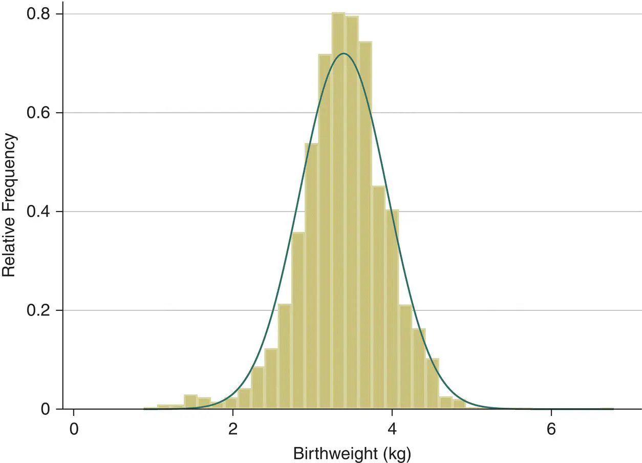
Figure 4.9 Distribution of birthweight in 3226 new‐born babies.
( Source: data from O'Cathain et al. 2002).
The histogram of the sample data is an estimate of the population distribution of birth weights in new‐born babies. This population distribution can be estimated by the superimposed smooth ‘bell‐shaped’ curve or ‘Normal’ distribution shown. We presume that if we were able to look at the entire population of new‐born babies then the distribution of birthweight would have exactly the Normal shape. The Normal distribution has the properties summarised in Figure 4.10.
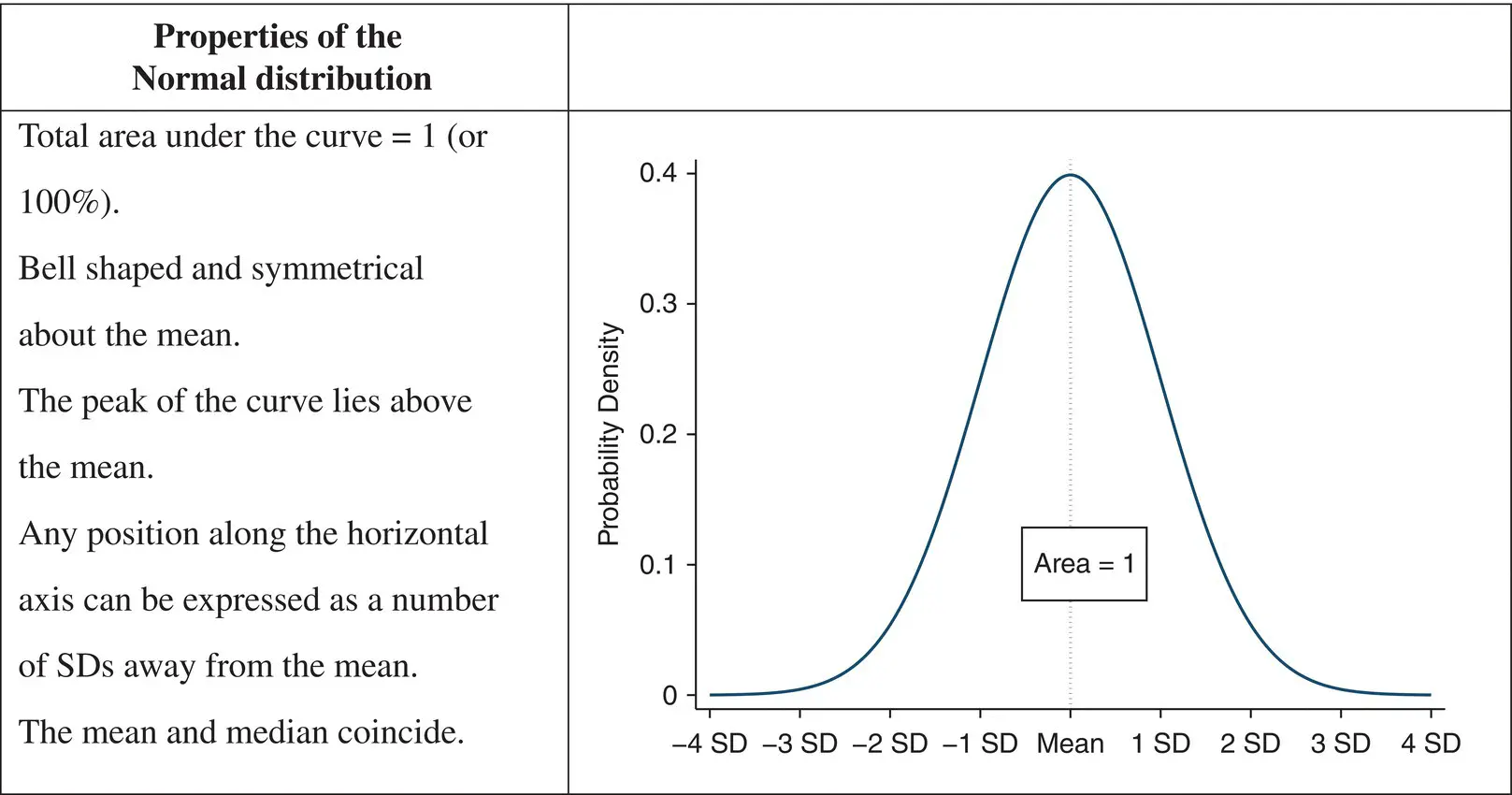
Figure 4.10 The Normal probability distribution.
The Normal distribution ( Figure 4.10), is completely described by two parameters: one, μ , represents the population mean or centre of the distribution and the other, σ , the population standard deviation. The formula for the Normal distribution is given as Eq. (4.3). Populations with small values of the standard deviation σ have a distribution concentrated close to the centre, μ ; those with large standard deviation have a distribution widely spread along the measurement axis ( Figure 4.11).
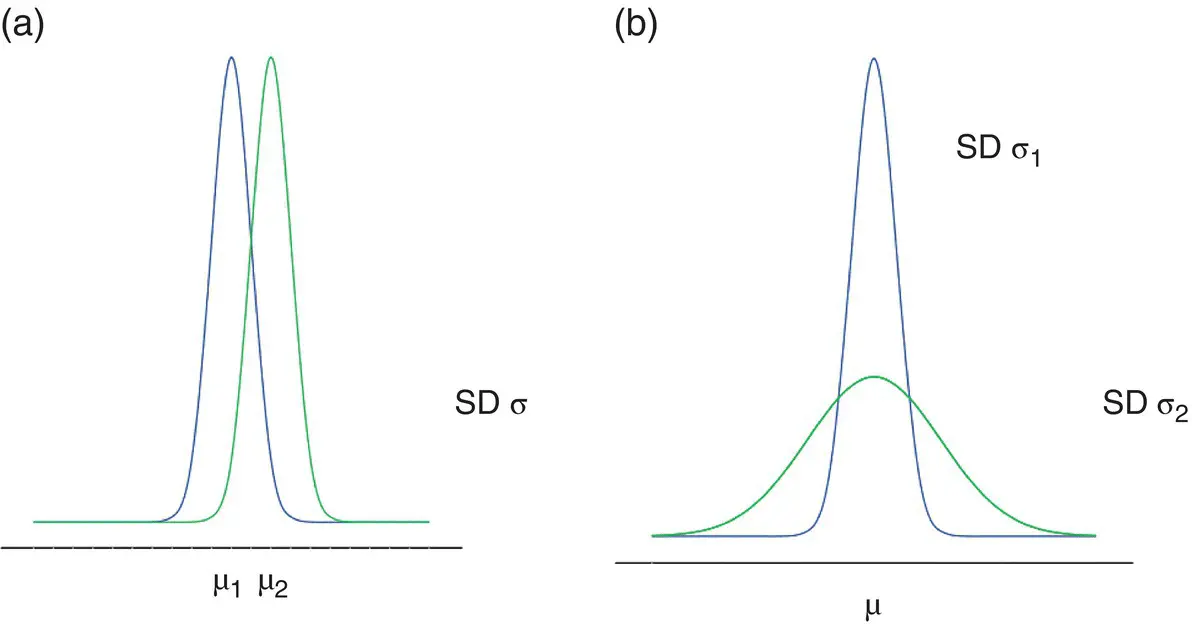
Figure 4.11 Probability distribution functions of the Normal distributions with different means and standard deviations. (a) Effect of changing mean (μ 2> μ 1). (b) Effect of changing SD (σ 2> σ 1).
There are infinitely many Normal distributions depending on the values of μ and σ . The Standard Normal distribution has a mean of zero and a variance (and standard deviation) of one and a shape as shown in Figure 4.10. The formula is given as Eq. (4.4)in Section 4.9. If the random variable X has a Normal distribution with mean, μ and standard deviation, σ, then the standardised Normal deviate  is a random variable that has a Standard Normal distribution.
The areas under the Standard Normal distribution curve have been tabulated in Table T1 in the appendix and some examples in Table 4.1. In column (i), the table gives for a positive value of Z , (that is the number of standard deviations above the mean of zero), the area under the Normal curve to the right of this value. The same value is obtained for the area below the same numerical, but negative, value − Z . Column (ii) gives the combination of these two equal areas. Using Figure 4.12or Table 4.1, we can note that much of the area (68%) of the probability is between −1 and +1 SD, the large majority (95%) between −2 and +2 SD, and almost all (99%) between −3 and +3.
Table 4.1 Selected probabilities associated with the Normal distribution.
| Standardised deviate | Probability of greater deviation | |
|---|---|---|
| Z = ( X − μ )/ σ | (i) Area in one direction | (ii) Area both directions |
| 0 | 0.5000 | 1.0000 |
| 1.000 | 0.1590 | 0.3170 |
| 1.645 | 0.0500 | 0.0100 |
| 1.960 | 0.0250 | 0.0500 |
| 2.000 | 0.0230 | 0.0460 |
| 2.576 | 0.0050 | 0.0100 |
| 3.000 | 0.0013 | 0.0027 |
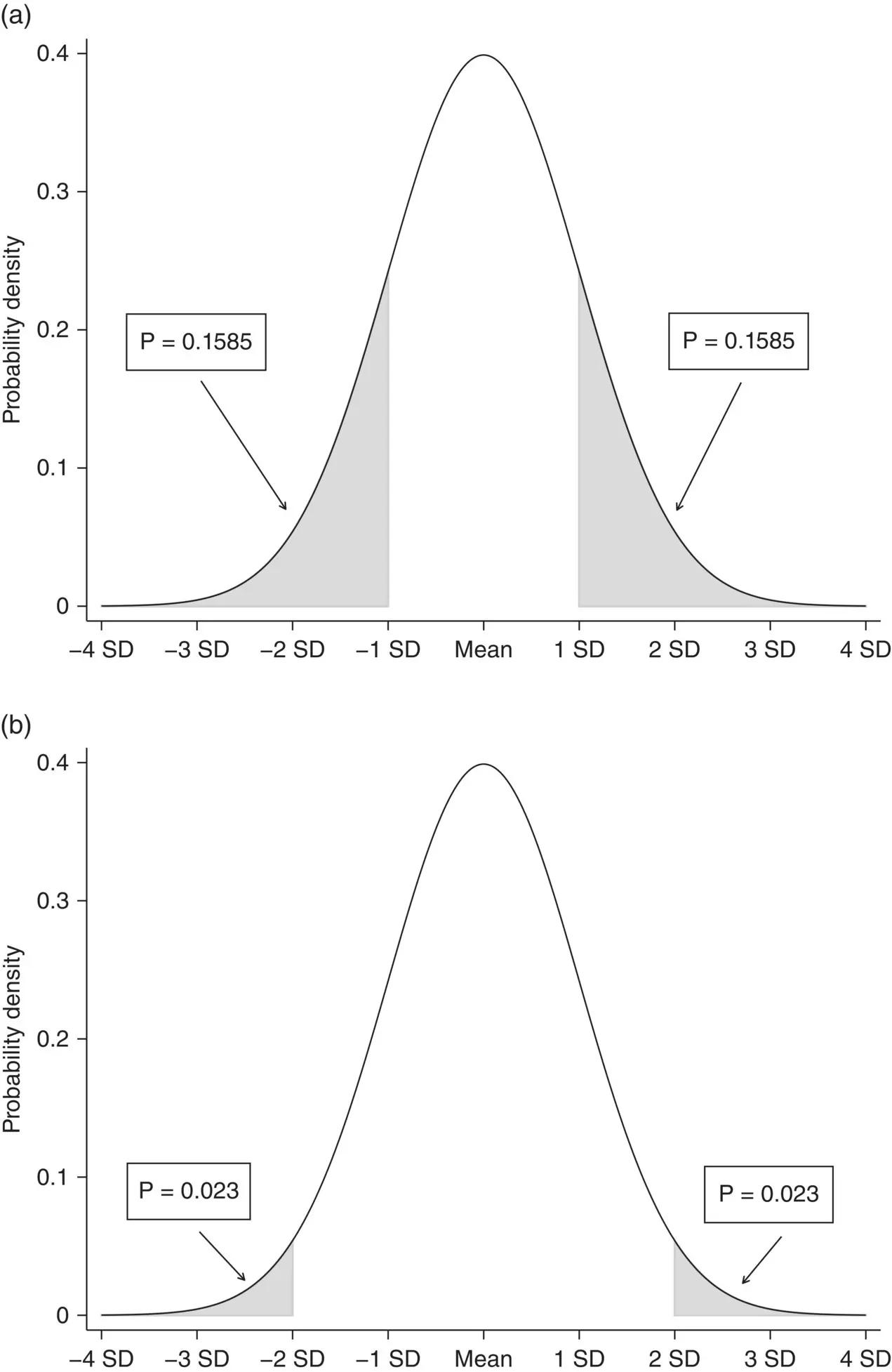
Figure 4.12 Areas (percentages of total probability) under the standard Normal curve. (a) 31.7% of observations lie outside the mean ± 1 SD. (b) 4.6% of observations lie outside the mean ± 2SD.
As can be seen from Table 4.1, using Z values of 1.96 (that is, 1.96 SD away from the mean) then exactly 95% of the Normal distribution lies between

Changing the multiplier 1.96 to 2.58, exactly 99% of the Normal distribution lies in the corresponding interval.
How Do We Use the Normal Distribution?
The Normal probability distribution can be used to calculate the probability of different values occurring. We could be interested in the probability of being within 1 SD of the mean (or outside it). We can use a Normal distribution table, which tells us the probability of being outside this value.
Illustrative Example – Normal Distribution – Birthweights
Using the birthweight data from the O'Cathain et al. (2002) study let us assume that the birthweight for new born babies has a Normal distribution with a mean of 3.4 kg and a standard deviation of 0.6 kg. So, what is the probability of giving birth to baby with a birthweight of 4.5 kg or higher?
Since birthweight is assumed to follow a Normal distribution, with mean of 3.4 kg and SD of 0.6 kg, we therefore know that approximately 68% of birthweights will lie between 2.8 and 4.0 kg and about 95% of birthweights will lie between 2.2 and 4.6 kg. Using Figure 4.13we can see that a birthweight of 4.5 kg is between one and two standard deviations away from the mean.
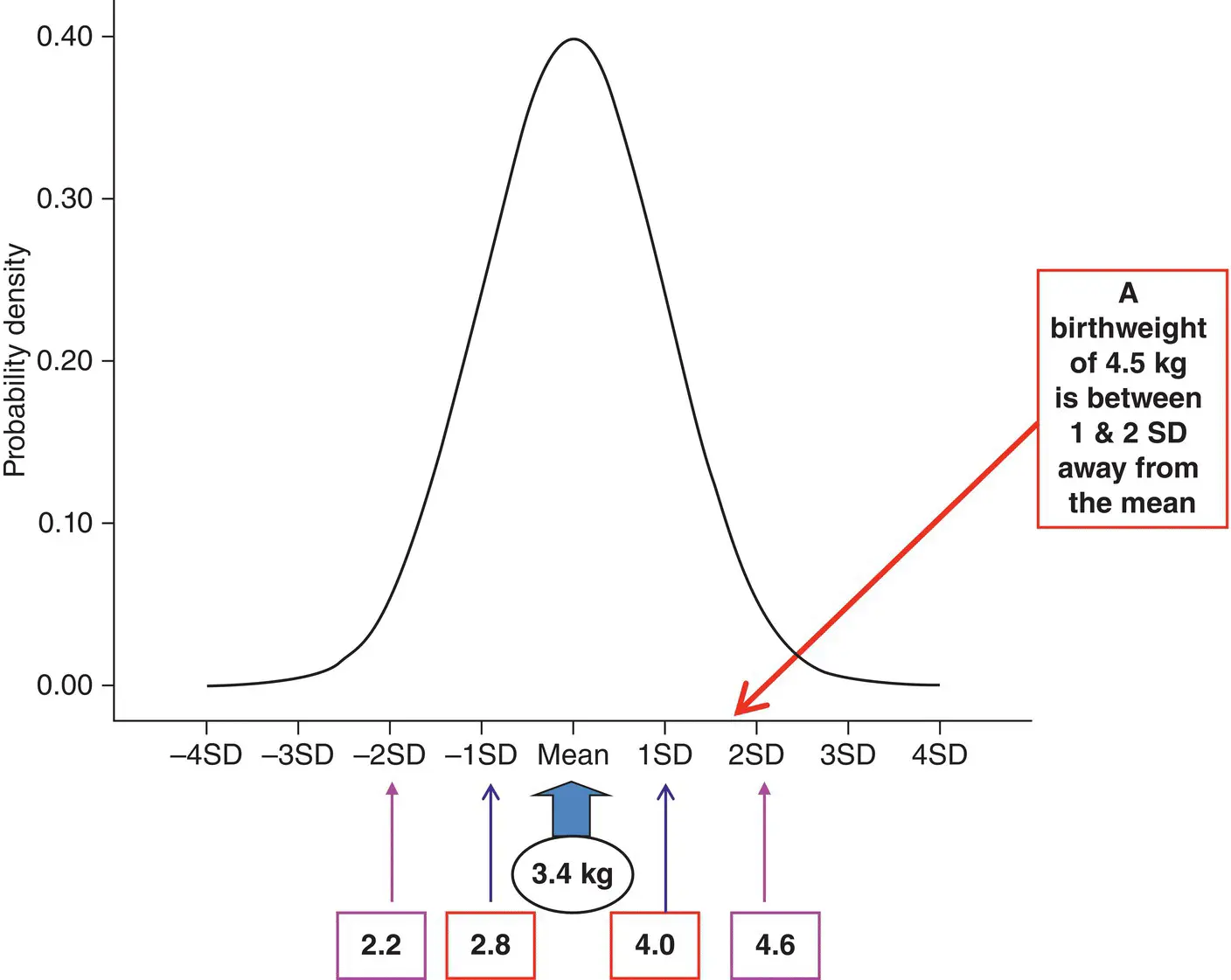
Figure 4.13 Normal distribution curve for birthweight with a mean of 3.4 kg and SD of 0.6 kg.
First calculate, Z , the number of standard deviations 4.5 kg is away from the mean of 3.4 kg, that is, 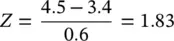 . Then look for z = 1.83 in Table T1 of the Normal distribution table, which gives the probability of being outside the values of the mean −1.83SD to mean +1.83SD as 0.0672. Therefore the probability of having a birthweight of 4.5 kg or higher is 0.0672/2 = 0.0336 or 3.4%.
The Normal distribution also has other uses in statistics and is often used as an approximation to the Binomial and Poisson distributions. Figure 4.4shows that the Binomial distribution for any particular value of the parameter π approaches the shape of a Normal distribution as the other parameter n increases. The approach to Normality is more rapid for values of π near 0.5 than for values near to 0 or 1. Thus, provided n is large enough, a count may be regarded as approximately Normally distributed with mean nπ and  . The Poisson distribution with mean λ approaches Normality as λ increases (see Figure 4.5). When λ is large a Poisson variable may be regarded as approximately Normally distributed with mean λ and SD = √λ.
Интервал:
Закладка:
Похожие книги на «Medical Statistics»
Представляем Вашему вниманию похожие книги на «Medical Statistics» списком для выбора. Мы отобрали схожую по названию и смыслу литературу в надежде предоставить читателям больше вариантов отыскать новые, интересные, ещё непрочитанные произведения.


Обсуждение, отзывы о книге «Medical Statistics» и просто собственные мнения читателей. Оставьте ваши комментарии, напишите, что Вы думаете о произведении, его смысле или главных героях. Укажите что конкретно понравилось, а что нет, и почему Вы так считаете.