David Machin - Medical Statistics

3 If two outcomes are independent (i.e. knowing the outcome of one experiment tells us nothing about the other experiment), then the probability of both occurring is the product of the individual probabilities (this is known as the ‘multiplication rule’).

When the outcome can never happen the probability is 0. When the outcome will definitely happen the probability is 1. If two events are mutually exclusive then only one can happen. For example, the outcome of a trial might be death (probability 5%) and severe disability (probability 20%). Thus, by the addition rule the probability of either death or severe disability is 25%.

If two events are independent then the fact that one has happened does not affect the chance of the other event happening. For example, the probability that a pregnant woman gives birth to a boy (event A) and the probability of white Christmas (event B). These two events are unconnected since the probability of giving birth to a boy is not related to the weather at Christmas.

If we throw a six‐sided die the probability of throwing a 6 is 1/6 and the probability of a 5 is also 1/6. We cannot throw a 5 and 6 at the same time (these events are mutually exclusive) using 1 die so the probability of throwing either 5 or a 6 is (by the addition rule):

Suppose we throw two six‐sided dice together. The probability of throwing a 6 is 1/6 for each die. The outcome of each die is independent of the other. Therefore, the probability of throwing two 6s together (by the multiplication rule) is:

If we toss a two‐sided coin it comes down either heads or tails. In a single toss of the coin you are uncertain whether you will get a head or a tail. However, if we carry on tossing our coin, we should get several heads and several tails. If we go on doing this for long enough, then we would expect to get as many heads as we do tails. So, the probability of a head being thrown is a half, because in the long run a head should occur on half the throws. The number of heads which might arise in several tosses of the coin is called a random variable , that is a variable which can take more than one value, each with a given probability attached to them.

If we toss a coin the two possibilities; head (H) – scored 1, or tail (T) – scored 0, are mutually exclusive and these are the only events which can happen. If we let X be a random variable that is the number of heads shown on a single toss and is therefore either 1 or 0, then the probability distribution, for X is: probability (H) = ½; probability (T) = ½ and is shown graphically in Figure 4.3a.

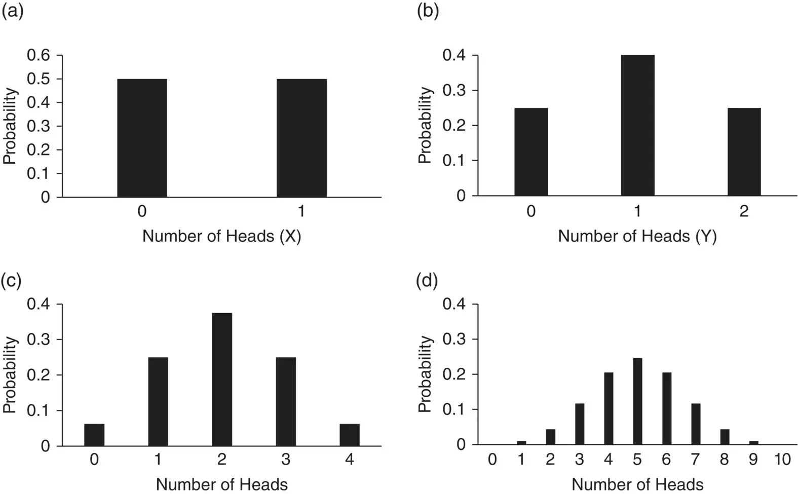
Figure 4.3 Examples of probability distributions. (a) Probability distribution for the number of heads ( X ) shown in one toss of a coin. (b) Probability distribution for the number of heads ( Y ) shown in two tosses of a coin. (c) Probability distribution for the number of heads in four tosses of a coin. (d) Probability distribution for the number of heads in ten tosses of a coin.

What happens if we toss two coins at once? We now have four possible events: HH, HT, TH, and TT. There are all equally likely and each has probability ¼. If we let Y be the number of heads then Y has three possible values 0, 1, and 2. Y = 0 only when we get TT and has probability ¼. Similarly, Y = 2 only when we get HH, so has probability ¼. However, Y = 1 either when we get HT or TH and so has probability ¼ + ¼ = ½. The probability distribution for Y is shown in Figure 4.3b. The distribution for the number of heads becomes more symmetrical as the number of coin tosses increases ( Figures 4.3c and d).

In general, we can think of the tosses of the coin as trials, each of which can have an outcome of success (H) or failure (T). These distributions are all examples of what is known as the Binomial distribution. In addition, we will discuss two more distributions that are the backbone of medical statistics: the Poisson and the Normal. Each of the distributions is known as the probability distribution function, which gives the probability of observing an event. The corresponding formulas are given in Section 4.7. These formulas contain certain constants, known as parameters, which identify the particular distribution, and from which various characteristics of the distribution, such as its mean and standard deviation, can be calculated.

If a group of patients is given a new treatment such as acupuncture for the relief of a particular condition, such as tension type headache, then the proportion p being successfully treated can be regarded as estimating the population treatment success rate π (here, π denotes a population value and has no connection at all with the mathematical constant 3.14159). The sample proportion p is analogous to the sample mean , in that if we score zero for those s patients who fail on treatment, and unity for those r who succeed, then p = r / n , where n = r + s is the total number of patients treated. The Binomial distribution is characterised by the parameters n (the number of individuals in the sample, or repetitions of the trial) and π (the true probability of success for each individual, or in each trial). The formula is given as Eq. (4.1)in Section 4.9.

For a fixed sample size n the shape of the Binomial distribution depends only on π. Suppose n = 5 patients are to be treated, and it is known that on average 0.25 will respond to this particular treatment. The number of responses actually observed can only take integer values between 0 (no responses) and 5 (all respond). The Binomial distribution for this case is illustrated in Figure 4.4a. The distribution is not symmetric; it has a maximum at one response and the height of the blocks corresponds to the probability of obtaining the particular number of responses from the five patients yet to be treated.

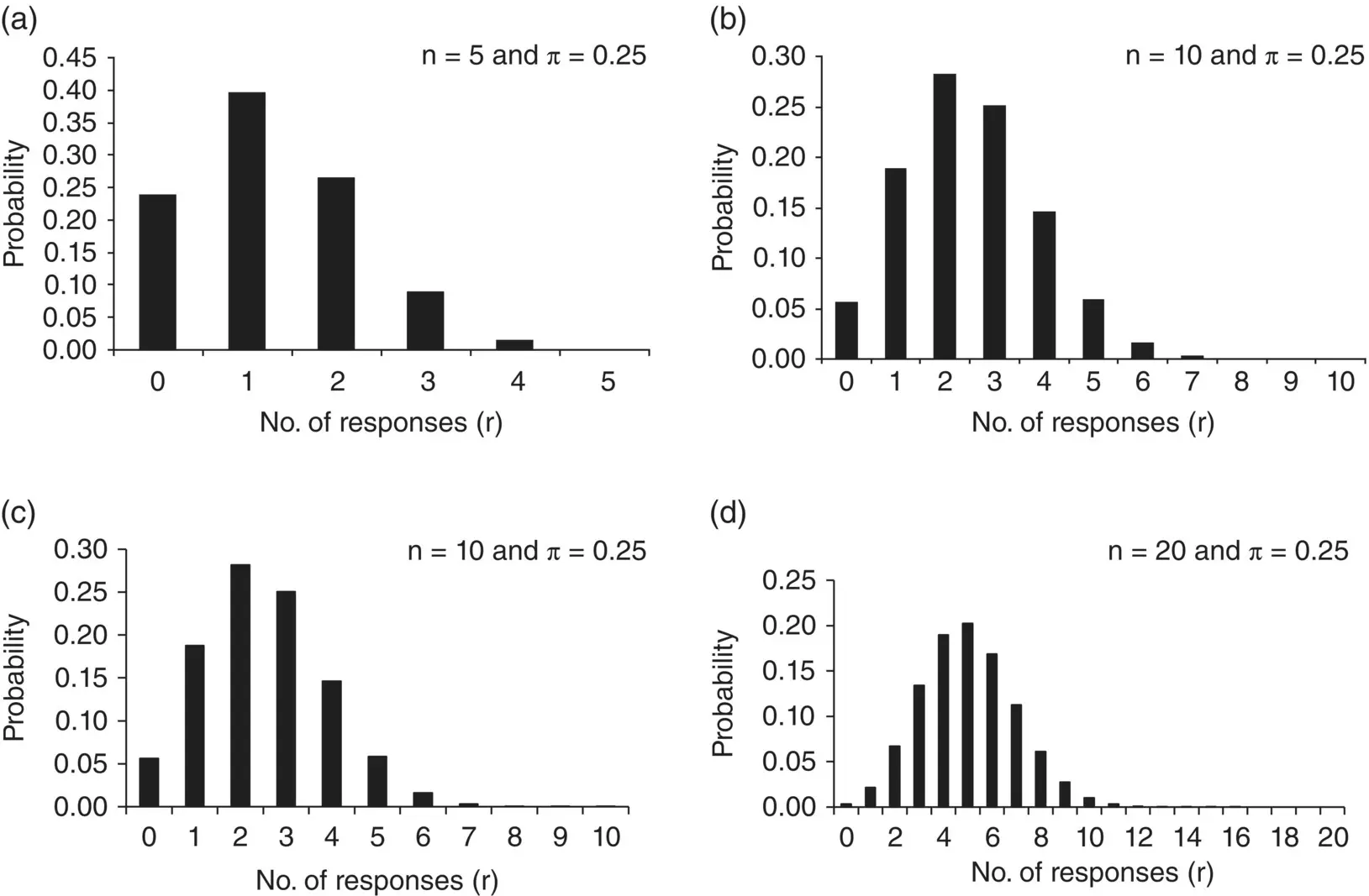
Figure 4.4 Binomial distribution for π = 0.25 and various values of n . The horizontal scale in each diagram shows the value of r the number of successes.

Figure 4.4illustrates the shape of the Binomial distribution for various n and π = 0.25. When n is small (here 5 and 10), as in Figure 4.4a and b, the distribution is skewed to the right. The distribution becomes more symmetrical as the sample size increases (here 20 and 50) as in Figure 4.4c and d. We also note that the width of the bars decreases as n increases since the total probability of unity is divided amongst more and more possibilities.