Francesca Lazzeri - Machine Learning for Time Series Forecasting with Python

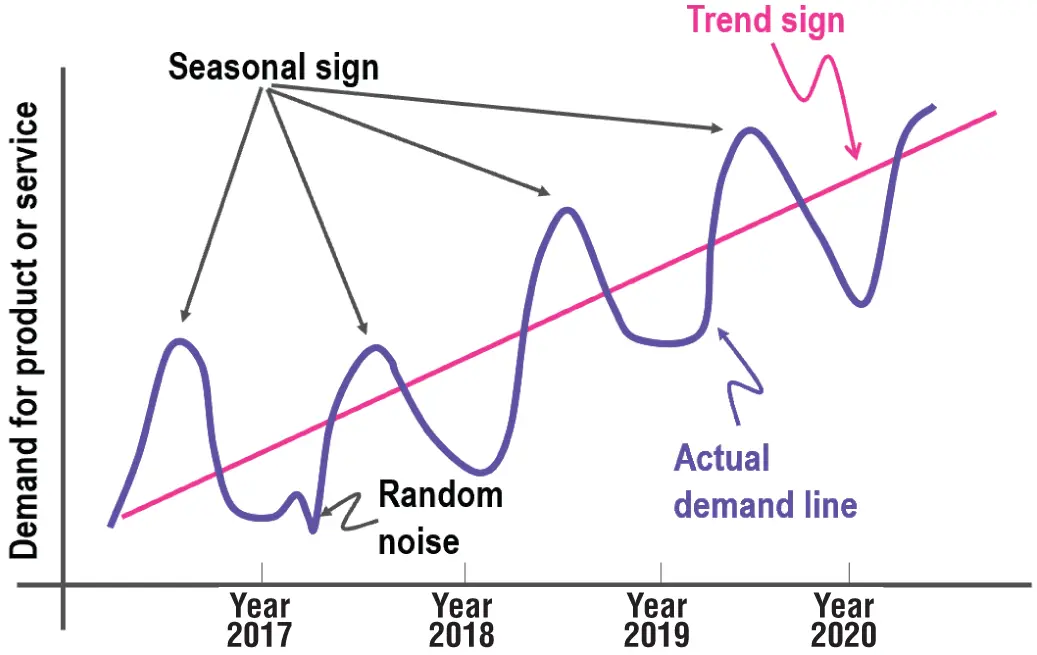
Figure 1.6 :Actual representation of time series components

Data scientists need to carefully identify to what extent each component is present in the time series data to be able to build an accurate machine learning forecasting solution. In order to recognize and measure these four components, it is recommended to first perform a decomposition process to remove the component effects from the data. After these components are identified and measured, and eventually utilized to build additional features to improve the forecast accuracy, data scientists can leverage different methods to recompose and add back the components on forecasted results.

Understanding these four time series components and how to identify and remove them represents a strategic first step for building any time series forecasting solution because they can help with another important concept in time series that may help increase the predictive power of your machine learning algorithms: stationarity. Stationarity means that statistical parameters of a time series do not change over time. In other words, basic properties of the time series data distribution, like the mean and variance, remain constant over time. Therefore, stationary time series processes are easier to analyze and model because the basic assumption is that their properties are not dependent on time and will be the same in the future as they have been in the previous historical period of time. Classically, you should make your time series stationary.

There are two important forms of stationarity: strong stationarity and weak stationarity . A time series is defined as having a strong stationarity when all its statistical parameters do not change over time. A time series is defined as having a weak stationarity when its mean and auto-covariance functions do not change over time.

Alternatively, time series that exhibit changes in the values of their data, such as a trend or seasonality, are clearly not stationary, and as a consequence, they are more difficult to predict and model. For accurate and consistent forecasted results to be received, the nonstationary data needs to be transformed into stationary data. Another important reason for trying to render a time series stationary is to be able to obtain meaningful sample statistics such as means, variances, and correlations with other variables that can be used to get more insights and better understand your data and can be included as additional features in your time series data set.

However, there are cases where unknown nonlinear relationships cannot be determined by classical methods, such as autoregression, moving average, and autoregressive integrated moving average methods. This information can be very helpful when building machine learning models, and it can be used in feature engineering and feature selection processes. In reality, many economic time series are far from stationary when visualized in their original units of measurement, and even after seasonal adjustment they will typically still exhibit trends, cycles, and other nonstationary characteristics.

Time series forecasting involves developing and using a predictive model on data where there is an ordered relationship between observations. Before data scientists get started with building their forecasting solution, it is highly recommended to define the following forecasting aspects:

The inputs and outputs of your forecasting model – For data scientists who are about to build a forecasting solution, it is critical to think about the data they have available to make the forecast and what they want to forecast about the future. Inputs are historical time series data provided to feed the model in order to make a forecast about future values. Outputs are the prediction results for a future time step. For example, the last seven days of energy consumption data collected by sensors in an electrical grid is considered input data, while the predicted values of energy consumption to forecast for the next day are defined as output data.

Granularity level of your forecasting model – Granularity in time series forecasting represents the lowest detailed level of values captured for each time stamp. Granularity is related to the frequency at which time series values are collected: usually, in Internet of Things (IoT) scenarios, data scientists need to handle time series data that has been collected by sensors every few seconds. IoT is typically defined as a group of devices that are connected to the Internet, all collecting, sharing, and storing data. Examples of IoT devices are temperature sensors in an air-conditioning unit and pressure sensors installed on a remote oil pump. Sometimes aggregating your time series data can represent an important step in building and optimizing your time series model: time aggregation is the combination of all data points for a single resource over a specified period (for example, daily, weekly, or monthly). With aggregation, the data points collected during each granularity period are aggregated into a single statistical value, such as the average or the sum of all the collected data points.

Horizon of your forecasting model – The horizon of your forecasting model is the length of time into the future for which forecasts are to be prepared. These generally vary from short-term forecasting horizons (less than three months) to long-term horizons (more than two years). Short-term forecasting is usually used in short-term objectives such as material requirement planning, scheduling, and budgeting; on the other hand, long-term forecasting is usually used to predict the long-term objectives covering more than five years, such as product diversification, sales, and advertising.

The endogenous and exogenous features of your forecasting model – Endogenous and exogenous are economic terms to describe internal and external factors, respectively, affecting business production, efficiency, growth, and profitability. Endogenous features are input variables that have values that are determined by other variables in the system, and the output variable depends on them. For example, if data scientists need to build a forecasting model to predict weekly gas prices, they can consider including major travel holidays as endogenous variables, as prices may go up because the cyclical demand is up.On the other hand, exogenous features are input variables that are not influenced by other variables in the system and on which the output variable depends. Exogenous variables present some common characteristics (Glen 2014), such as these:They are fixed when they enter the model.They are taken as a given in the model.They influence endogenous variables in the model.They are not determined by the model.They are not explained by the model.In the example above of predicting weekly gas prices, while the holiday travel schedule increases demand based on cyclical trends, the overall cost of gasoline could be affected by oil reserve prices, sociopolitical conflicts, or disasters such as oil tanker accidents.

The structured or unstructured features of your forecasting model – Structured data comprises clearly defined data types whose pattern makes them easily searchable, while unstructured data comprises data that is usually not as easily searchable, including formats like audio, video, and social media postings. Structured data usually resides in relational databases, whose fields store length delineated data such as phone numbers, Social Security numbers, or ZIP codes. Even text strings of variable length like names are contained in records, making it a simple matter to search (Taylor 2018).Unstructured data has internal structure but is not structured via predefined data models or schema. It may be textual or non-textual, and human or machine generated. Typical human-generated unstructured data includes spreadsheets, presentations, email, and logs. Typical machine-generated unstructured data includes satellite imagery, weather data, landforms, and military movements.In a time series context, unstructured data doesn't present systematic time-dependent patterns, while structured data shows systematic time dependent patterns, such as trend and seasonality.