Francesca Lazzeri - Machine Learning for Time Series Forecasting with Python

Due to their applicability to many real-life problems, such as fraud detection, spam email filtering, finance, and medical diagnosis, and their ability to produce actionable results, machine learning and deep learning algorithms have gained a lot of attention in recent years. Generally, deep learning methods have been developed and applied to univariate time series forecasting scenarios, where the time series consists of single observations recorded sequentially over equal time increments (Lazzeri 2019a).

For this reason, they have often performed worse than naïve and classical forecasting methods, such as exponential smoothing and autoregressive integrated moving average (ARIMA). This has led to a general misconception that deep learning models are inefficient in time series forecasting scenarios, and many data scientists wonder whether it's really necessary to add another class of methods, such as convolutional neural networks (CNNs) or recurrent neural networks (RNNs), to their time series toolkit (we will discuss this in more detail in Chapter 5, “Introduction to Neural Networks for Time Series Forecasting”) (Lazzeri 2019a).

In time series, the chronological arrangement of data is captured in a specific column that is often denoted as time stamp , date , or simply time . As illustrated in Figure 1.2, a machine learning data set is usually a list of data points containing important information that are treated equally from a time perspective and are used as input to generate an output, which represents our predictions. On the contrary, a time structure is added to your time series data set, and all data points assume a specific value that is articulated by that temporal dimension.

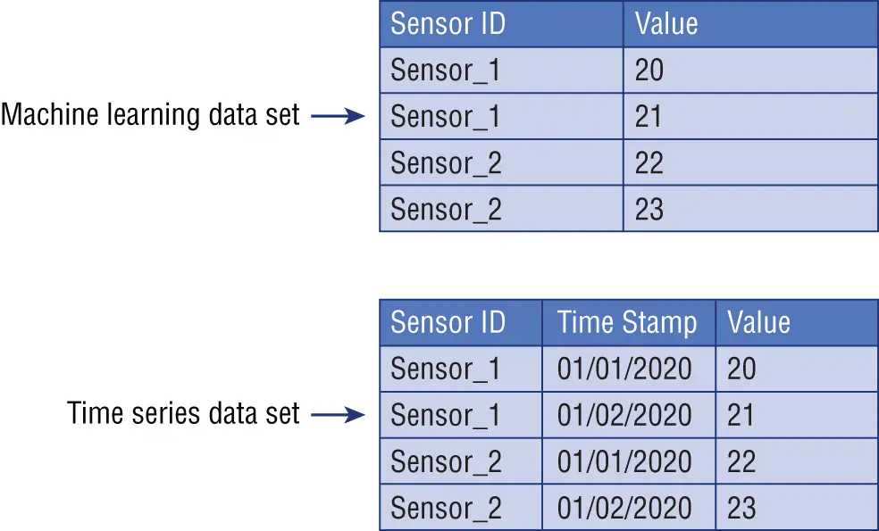
Figure 1.2 :Machine learning data set versus time series data set

Now that you have a better understanding of time series data, it is also important to understand the difference between time series analysis and time series forecasting. These two domains are tightly related, but they serve different purposes: time series analysis is about identifying the intrinsic structure and extrapolating the hidden traits of your time series data in order to get helpful information from it (like trend or seasonal variation—these are all concepts that we will discuss later on in the chapter).

Data scientists usually leverage time series analysis for the following reasons:

Acquire clear insights of the underlying structures of historical time series data.

Increase the quality of the interpretation of time series features to better inform the problem domain.

Preprocess and perform high-quality feature engineering to get a richer and deeper historical data set.

Time series analysis is used for many applications such as process and quality control, utility studies, and census analysis. It is usually considered the first step to analyze and prepare your time series data for the modeling step, which is properly called time series forecasting .

Time series forecasting involves taking machine learning models, training them on historical time series data, and consuming them to forecast future predictions. As illustrated in Figure 1.3, in time series forecasting that future output is unknown, and it is based on how the machine learning model is trained on the historical input data.

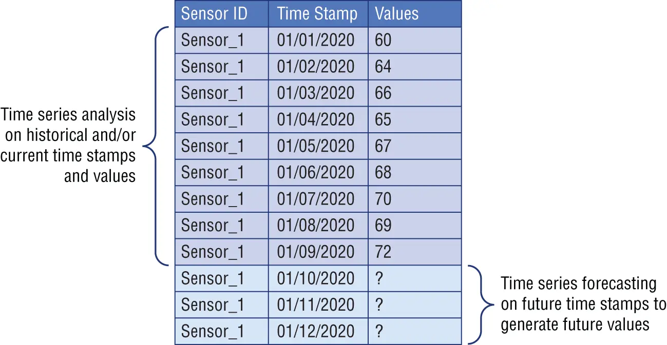
Figure 1.3 :Difference between time series analysis historical input data and time series forecasting output data

Different historical and current phenomena may affect the values of your data in a time series, and these events are diagnosed as components of a time series. It is very important to recognize these different influences or components and decompose them in order to separate them from the data levels.

As illustrated in Figure 1.4, there are four main categories of components in time series analysis: long-term movement or trend , seasonal short-term movements , cyclic short-term movements , and random or irregular fluctuations .

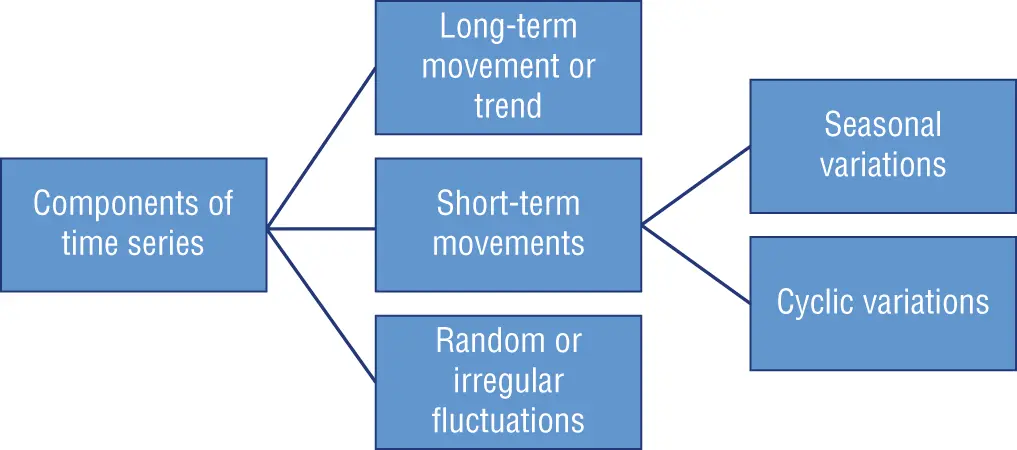
Figure 1.4 :Components of time series

Let's have a closer look at these four components:

Long-term movement or trend refers to the overall movement of time series values to increase or decrease during a prolonged time interval. It is common to observe trends changing direction throughout the course of your time series data set: they may increase, decrease, or remain stable at different moments. However, overall you will see one primary trend. Population counts, agricultural production, and items manufactured are just some examples of when trends may come into play.

There are two different types of short-term movements:Seasonal variations are periodic temporal fluctuations that show the same variation and usually recur over a period of less than a year. Seasonality is always of a fixed and known period. Most of the time, this variation will be present in a time series if the data is recorded hourly, daily, weekly, quarterly, or monthly. Different social conventions (such as holidays and festivities), weather seasons, and climatic conditions play an important role in seasonal variations, like for example the sale of umbrellas and raincoats in the rainy season and the sale of air conditioners in summer seasons.Cyclic variations, on the other side, are recurrent patterns that exist when data exhibits rises and falls that are not of a fixed period. One complete period is a cycle, but a cycle will not have a specific predetermined length of time, even if the duration of these temporal fluctuations is usually longer than a year. A classic example of cyclic variation is a business cycle, which is the downward and upward movement of gross domestic product around its long-term growth trend: it usually can last several years, but the duration of the current business cycle is unknown in advance.As illustrated in Figure 1.5, cyclic variations and seasonal variations are part of the same short-term movements in time series forecasting, but they present differences that data scientists need to identify and leverage in order to build accurate forecasting models: Figure 1.5 : Differences between cyclic variations versus seasonal variations

Random or irregular fluctuations are the last element to cause variations in our time series data. These fluctuations are uncontrollable, unpredictable, and erratic, such as earthquakes, wars, flood, and any other natural disasters.

Data scientists often refer to the first three components (long-term movements, seasonal short-term movements, and cyclic short-term movements) as signals in time series data because they actually are deterministic indicators that can be derived from the data itself. On the other hand, the last component (random or irregular fluctuations) is an arbitrary variation of the values in your data that you cannot really predict, because each data point of these random fluctuations is independent of the other signals above, such as long-term and short-term movements. For this reason, data scientists often refer to it as noise , because it is triggered by latent variables difficult to observe, as illustrated in Figure 1.6.