Data Analytics in Bioinformatics
Здесь есть возможность читать онлайн «Data Analytics in Bioinformatics» — ознакомительный отрывок электронной книги совершенно бесплатно, а после прочтения отрывка купить полную версию. В некоторых случаях можно слушать аудио, скачать через торрент в формате fb2 и присутствует краткое содержание. Жанр: unrecognised, на английском языке. Описание произведения, (предисловие) а так же отзывы посетителей доступны на портале библиотеки ЛибКат.
- Название:Data Analytics in Bioinformatics
- Автор:
- Жанр:
- Год:неизвестен
- ISBN:нет данных
- Рейтинг книги:5 / 5. Голосов: 1
-
Избранное:Добавить в избранное
- Отзывы:
-
Ваша оценка:
Data Analytics in Bioinformatics: краткое содержание, описание и аннотация
Предлагаем к чтению аннотацию, описание, краткое содержание или предисловие (зависит от того, что написал сам автор книги «Data Analytics in Bioinformatics»). Если вы не нашли необходимую информацию о книге — напишите в комментариях, мы постараемся отыскать её.
Data Analytics in Bioinformatics — читать онлайн ознакомительный отрывок
Ниже представлен текст книги, разбитый по страницам. Система сохранения места последней прочитанной страницы, позволяет с удобством читать онлайн бесплатно книгу «Data Analytics in Bioinformatics», без необходимости каждый раз заново искать на чём Вы остановились. Поставьте закладку, и сможете в любой момент перейти на страницу, на которой закончили чтение.
Интервал:
Закладка:
The Logistic Regression is performed on the heart disease dataset [41]. The Receiver Operating Characteristics (ROC) is calculated that is based on the true positive rate that is plotted on the y-axis and the false positive rate that is plotted on the x-axis. After performing the logistic regression in python (Google Colab), the outcome is represented in Figure 1.11 and Table 1.2. Figure 1.11 represents the ROC curve and Table 1.2 represents the Area under the ROC Curve (AUC).
At the time of processing, the AUC value obtained (Table 1.2) on training data is 0.8374022, but when the data is processed for testing then the obtained result is outstanding (i.e. 0.9409523). This indicates that the model is more than 90% efficient for classification. In the next section, the difference between Linear and Logistic Regression is discussed.
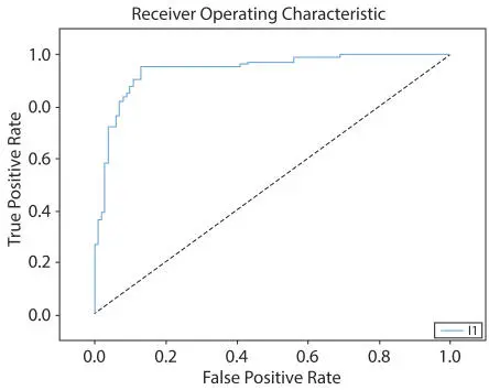
Figure 1.11 ROC curve for logistic regression.
Table 1.2AUC: Logistic regression.
| Parameter | Data | Value | Result |
| The area under | Training Data | 0.8374022 | Excellent |
| the ROC Curve (AUC) | Test Data | 0.9409523 | Outstanding |
| Index: 0.5: No Discriminant, 0.6–0.8: Can be considered accepted, 0.8–0.9: Excellent, >0.9: Outstanding |
1.4.2 Difference between Linear & Logistic Regression
Linear and Logistics regression are two common types of regression used for prediction. The result of the prediction is represented with the help of numeric variables. The difference between linear and logistic regression is depicted in Table 1.3 for easy understanding.
Linear regression is used to model the data by using a straight line whereas the logistic regression deals with the modeling of probability of events in a bi-variate manner that is occurring as a linear function of dependent variables. Few other types of regression analysis are depicted by different scientists and listed below.
Table 1.3Difference between linear & logistic regression.
| S. No. | Parameter | Linear regression | Logistic regression |
| 1 | Purpose | Used for solving regression problems. | Used for solving classification problems. |
| 2 | Variables Involved | Continuous Variables | Categorical Variables |
| 3 | Objective | Finding of best-fit-line and predicting the output. | Finding of s-curve and classifying the samples. |
| 4 | Output | Continuous Variables such as age, price, etc. | Categorical Values such as 0 & 1, Yes & No. |
| 5 | Collinearity | There may be collinearity between independent attributes. | There should not be collinearity between independent attributes. |
| 6 | Relationship | The relationship between a dependent variable and the independent variable must be linear. | The relationship between a dependent variable and an independent variable may not be linear. |
| 7 | Estimation Method Used | Least Square Estimation | Maximum Likelihood Estimation |
Polynomial Regression: It is used for curvilinear data [57–58].
Stepwise Regression: It works with predictive models [59–60].
Ridge Regression: Used for multiple regression data [61–62].
Lasso Regression: Used for the purpose of variable selection & regularization [63–64].
Elastic Net Regression: Used when the penalties of lasso and ridge method are combined [65].
1.5 Random Forest
The Random Forest was first invented by Tim Kan Ho [66]. Random Forest is a supervised ensemble learning method, which solves regression and classification problems. It is a method of ensemble learning (i.e. bagging algorithm) and works by averaging the result and by reducing overfitting [67–71]. It is a flexible method and a ready to use in the machine learning algorithm. The Random Forest can be used for the process of regression and known as Regression Forests [72]. It can cope up with the missing values but deals with complexity as well as a longer training period. There are two specific causes for naming it as Random that are:
When building trees, then a random sampling of training data sets is followed.
When Splitting nodes, then a random subset of features is considered.
The functioning of random forests is illustrated in Figure 1.12.
In the above figure, five forests are there and each one representing a disease, such as blue represents liver disease, orange represents heart disease, the green tree represents stomach disease, yellow represents lung disease. It was observed that as per the majority of color, Orange is the winner.
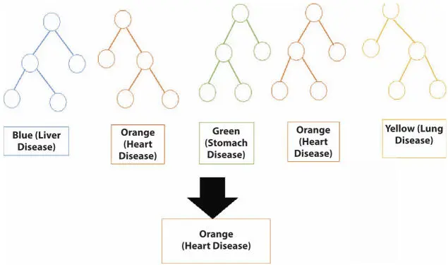
Figure 1.12Random forest.
This concept is known as the Wisdom of crowd as discussed in Ref. [73]. The execution of this method is achieved with the help of two concepts, which is listed below
Bagging: The Data on which the decision trees are trained are very sensitive. This means a small change in the data can bring diverse effects in the model. Because of this, the structure of the tree can completely change. They take benefit of it by allowing each tree to randomly sample the dataset with a replacement that results in different trees. This is called bagging or bootstrap aggregation [74–75].
Random Feature Selection: Normally, when we split a node, every possible feature is considered. The one that produces the most separation is considered. Whereas, in the random forest scenario we can consider a random subset of features. This allows more variation in the model and results in a greater diversification. [76]
The Concept of Random Forest took place in the heart disease dataset also. The low correlation is the key, between the models. The Area under the ROC Curve (AUC) characteristic of Random Forest performed in python (Google Colab) is shown in Table 1.4 and Figure 1.13.
In the above table, the area under the receiver operating characteristic curve (AUC) is mentioned.
AUC measures the degree of separability. The obtained value of Training Data is 1.0000000 that attains an outstanding remark and the value of the testing data is 1.0000000 that attains an outstanding remark in the AUC score. The result indicates that the used models perform outstandingly on the heart disease dataset.
Table 1.4AUC: Random forest.
| Parameter | Data | Value | Result |
| The area under the ROC Curve (AUC) | Training Data | 1.0000000 | Outstanding |
| Test Data | 1.0000000 | Outstanding | |
| Index: 0.5: No Discriminant, 0.6–0.8: Can be considered accepted, 0.8–0.9: Excellent, >0.9: Outstanding |
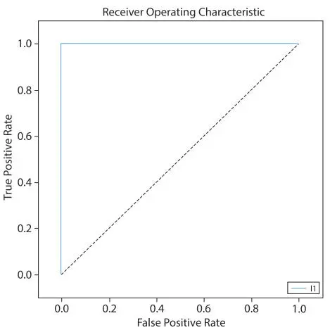
Figure 1.13ROC curve for random forest.
Читать дальшеИнтервал:
Закладка:
Похожие книги на «Data Analytics in Bioinformatics»
Представляем Вашему вниманию похожие книги на «Data Analytics in Bioinformatics» списком для выбора. Мы отобрали схожую по названию и смыслу литературу в надежде предоставить читателям больше вариантов отыскать новые, интересные, ещё непрочитанные произведения.


Обсуждение, отзывы о книге «Data Analytics in Bioinformatics» и просто собственные мнения читателей. Оставьте ваши комментарии, напишите, что Вы думаете о произведении, его смысле или главных героях. Укажите что конкретно понравилось, а что нет, и почему Вы так считаете.