Caner Ozdemir - Inverse Synthetic Aperture Radar Imaging With MATLAB Algorithms
Здесь есть возможность читать онлайн «Caner Ozdemir - Inverse Synthetic Aperture Radar Imaging With MATLAB Algorithms» — ознакомительный отрывок электронной книги совершенно бесплатно, а после прочтения отрывка купить полную версию. В некоторых случаях можно слушать аудио, скачать через торрент в формате fb2 и присутствует краткое содержание. Жанр: unrecognised, на английском языке. Описание произведения, (предисловие) а так же отзывы посетителей доступны на портале библиотеки ЛибКат.
- Название:Inverse Synthetic Aperture Radar Imaging With MATLAB Algorithms
- Автор:
- Жанр:
- Год:неизвестен
- ISBN:нет данных
- Рейтинг книги:5 / 5. Голосов: 1
-
Избранное:Добавить в избранное
- Отзывы:
-
Ваша оценка:
Inverse Synthetic Aperture Radar Imaging With MATLAB Algorithms: краткое содержание, описание и аннотация
Предлагаем к чтению аннотацию, описание, краткое содержание или предисловие (зависит от того, что написал сам автор книги «Inverse Synthetic Aperture Radar Imaging With MATLAB Algorithms»). Если вы не нашли необходимую информацию о книге — напишите в комментариях, мы постараемся отыскать её.
covers in greater detail the fundamental and advanced topics necessary for a complete understanding of inverse synthetic aperture radar (ISAR) imaging and its concepts. Distinguished author and academician, Caner Özdemir, describes the practical aspects of ISAR imaging and presents illustrative examples of the radar signal processing algorithms used for ISAR imaging. The topics in each chapter are supplemented with MATLAB codes to assist readers in better understanding each of the principles discussed within the book.
This new edition incudes discussions of the most up-to-date topics to arise in the field of ISAR imaging and ISAR hardware design. The book provides a comprehensive analysis of advanced techniques like Fourier-based radar imaging algorithms, and motion compensation techniques along with radar fundamentals for readers new to the subject.
The author covers a wide variety of topics, including:
Radar fundamentals, including concepts like radar cross section, maximum detectable range, frequency modulated continuous wave, and doppler frequency and pulsed radar The theoretical and practical aspects of signal processing algorithms used in ISAR imaging The numeric implementation of all necessary algorithms in MATLAB ISAR hardware, emerging topics on SAR/ISAR focusing algorithms such as bistatic ISAR imaging, polarimetric ISAR imaging, and near-field ISAR imaging, Applications of SAR/ISAR imaging techniques to other radar imaging problems such as thru-the-wall radar imaging and ground-penetrating radar imaging Perfect for graduate students in the fields of electrical and electronics engineering, electromagnetism, imaging radar, and physics,
also belongs on the bookshelves of practicing researchers in the related areas looking for a useful resource to assist them in their day-to-day professional work.
Inverse Synthetic Aperture Radar Imaging With MATLAB Algorithms — читать онлайн ознакомительный отрывок
Ниже представлен текст книги, разбитый по страницам. Система сохранения места последней прочитанной страницы, позволяет с удобством читать онлайн бесплатно книгу «Inverse Synthetic Aperture Radar Imaging With MATLAB Algorithms», без необходимости каждый раз заново искать на чём Вы остановились. Поставьте закладку, и сможете в любой момент перейти на страницу, на которой закончили чтение.
Интервал:
Закладка:
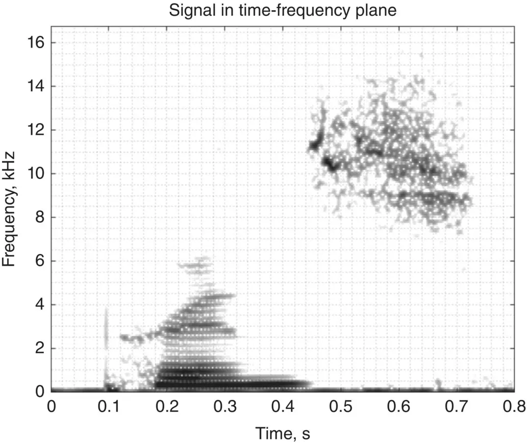
Figure 1.3 The time‐frequency representation of the word “prince.”
An example of the use of spectrogram is demonstrated in Figure 1.3. The spectrogram of the sound signal in Figure 1.1is obtained by applying the STFT operation with a Hanning window. This JFT representation obviously demonstrates the frequency content of different syllables when the word “prince” is spoken. Figure 1.3illustrates that while the frequency content of the part “prin…” takes place at low frequencies, that of the part “..ce” occurs at much higher frequencies.
JTF transformation tools have been found to be very useful in interpreting the physical mechanisms such as scattering and resonance for radar applications (Trintinalia and Ling 1995; Filindras et al. 1996; Özdemir and Ling 1997; Chen and Ling 2002). In particular, when JTF transforms are used to form the 2D image of electromagnetic scattering from various structures, many useful physical features can be displayed. Distinct time events (such as scattering from point targets or specular points) show up as vertical line in the JTF plane as depicted in Figure 1.4a. Therefore, these scattering centers appear at only one time instant but for all frequencies. A resonance behavior such as scattering from an open cavity structure shows up as horizontal line on the JTF plane. Such mechanisms occur only at discrete frequencies but over all time instants (see Figure 1.4b). Dispersive mechanisms, on the other hand, are represented on the JTF plane as slanted curves. If the dispersion is due to the material, then the slope of the image is positive as shown in Figure 1.4c,d. The dielectric coated structures are the good examples of this type of dispersion. The reason for having a slanted line is because of the modes excited inside such materials. As frequency increases, the wave velocity changes for different modes inside these materials. Consequently, these modes show up as slanted curves in the JTF plane. Finally, if the dispersion is due to the geometry of the structure, this type of mechanism appears as a slanted line with a negative slope. This style of behavior occurs for such structures such as waveguides where there exist different modes with different wave velocities as the frequency changes as seen in Figure 1.4e,f.
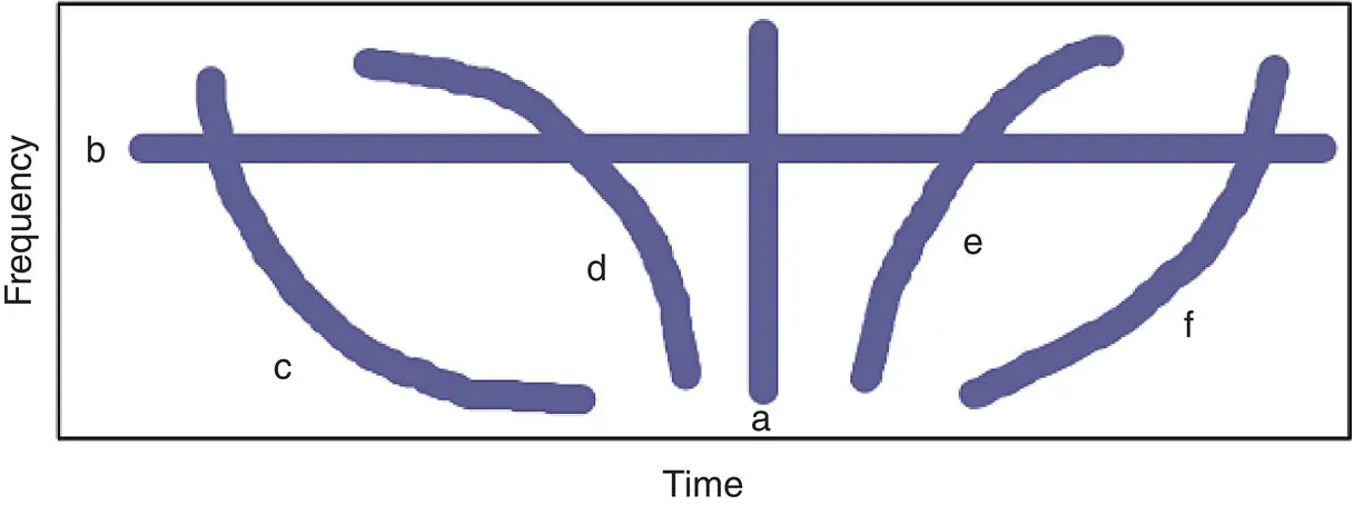
Figure 1.4 Images of scattering mechanisms in the joint time–frequency plane. (a) Scattering center, (b) resonance, (c and d) dispersion due to material, (e and f) dispersion due to geometry of the structure.
An example of the use of JTF processing in radar application is shown in Figure 1.5where spectrogram of the simulated backscattered data from a dielectric‐coated wire antenna is shown (Özdemir and Ling 1997). The backscattered field is collected from the Teflon‐coated wire ( ε r= 2.1) such that the tip of the electric field makes an angle of 60° with the wire axis as illustrated in Figure 1.5. After the incident field hits the wire, infinitely successive scattering mechanisms occur. The first four of them are illustrated on top of Figure 1.5. The first return comes from the near tip of the wire. This event occurs at a discrete time that exists at all frequencies. Therefore, this return demonstrates a scattering center‐type mechanism. On the other hand, all other returns experience at least one trip along the dielectric‐coated wire. Therefore, they confront a dispersive behavior. As the wave travels along the dielectric‐coated wire, it is influenced by the dominant dispersive surface mode called Goubau (Richmond and Newman 1976). Therefore, the wave velocity decreases as the frequency increases such that the dispersive returns are tilted to later times on the JTF plane. The dominant dispersive scattering mechanisms numbered 2, 3, and 4 are illustrated in Figure 1.5where the spectrogram of the backscattered field is presented. The other dispersive returns with decreasing energy levels can also be easily observed from the spectrogram plot. As the wave travels on the dielectric‐coated wire more and more, it is slanted more on the JTF plane, as expected.
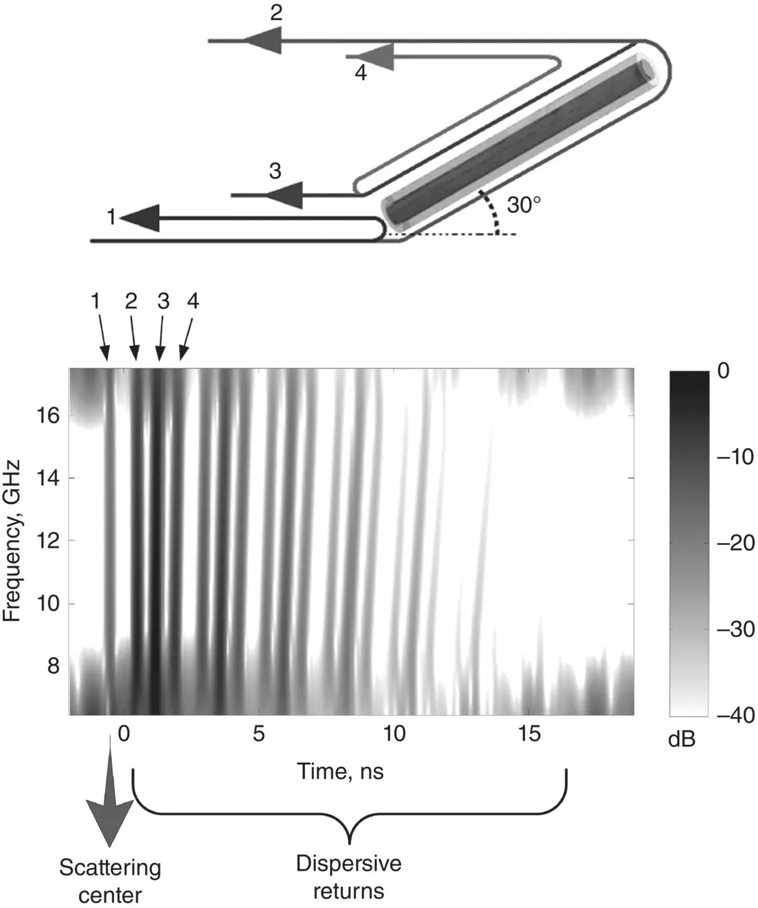
Figure 1.5 JTF image of a backscattered measured data from a dielectric‐coated wire antenna using spectrogram.
1.4 Convolution and Multiplication Using FT
Convolution and multiplication of signals are often used in radar signal processing. As listed in Eqs. 1.12and 1.13, convolution is the inverse operation of multiplication as the FT is concerned, and vice versa. This useful feature of the FT is widely used in signal and image processing applications. It is obvious that the multiplication operation is significantly faster and easier to deal with when compared to the convolution operation, especially for long signals. Instead of directly convolving two signals in the time domain, therefore, it is much easier and faster to take the IFT of the multiplication of the spectrums of those signals as shown below:
(1.18) 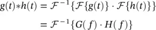
In a dual manner, convolution between the frequency‐domain signals can be calculated in a much faster and easier way by taking the FT of the product of their time‐domain versions as formulated below:
(1.19) 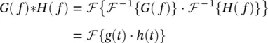
1.5 Filtering/Windowing
Filtering is the common procedure that is used to remove undesired parts of signals such as noise. It is also used to extract some useful features of the signals. The filtering function is usually in the form of a window in the frequency domain. Depending on the frequency inclusion of the window in the frequency axis, the filters are named low‐pass (LP), high‐pass (HP), or band‐pass (BP).
The frequency characteristics of an ideal LP filter are depicted as dashed line in Figure 1.6. Ideally, this filter should pass frequencies from DC to the cut‐off frequency; f cand should stop higher frequencies beyond. In real practice, however, ideal LP filter characteristics cannot be realized. According to the Fourier theory, a signal cannot be both time limited and band limited . That is to say, to be able to achieve an ideal band‐limited characteristic as in Figure 1.6, then the corresponding time‐domain signal should theoretically extent to infinity which is of course not possible for realistic applications. Since all practical human‐made signals are time limited, i.e. it should start and stop at specific time instants, the frequency contents of these signals extent to infinity. Therefore, an ideal filter characteristic as the one in Figure 1.6cannot be realizable; but, only the approximate versions of it can be implemented in real applications. The best implementation of practical low‐pass filter characteristic was achieved by Butterworth (Daniels 1974) and Chebyshev (Williams and Taylors 1988). The solid line in Figure 1.6demonstrates a real LP filter characteristic of Butterworth type.
Читать дальшеИнтервал:
Закладка:
Похожие книги на «Inverse Synthetic Aperture Radar Imaging With MATLAB Algorithms»
Представляем Вашему вниманию похожие книги на «Inverse Synthetic Aperture Radar Imaging With MATLAB Algorithms» списком для выбора. Мы отобрали схожую по названию и смыслу литературу в надежде предоставить читателям больше вариантов отыскать новые, интересные, ещё непрочитанные произведения.


Обсуждение, отзывы о книге «Inverse Synthetic Aperture Radar Imaging With MATLAB Algorithms» и просто собственные мнения читателей. Оставьте ваши комментарии, напишите, что Вы думаете о произведении, его смысле или главных героях. Укажите что конкретно понравилось, а что нет, и почему Вы так считаете.