Caner Ozdemir - Inverse Synthetic Aperture Radar Imaging With MATLAB Algorithms
Здесь есть возможность читать онлайн «Caner Ozdemir - Inverse Synthetic Aperture Radar Imaging With MATLAB Algorithms» — ознакомительный отрывок электронной книги совершенно бесплатно, а после прочтения отрывка купить полную версию. В некоторых случаях можно слушать аудио, скачать через торрент в формате fb2 и присутствует краткое содержание. Жанр: unrecognised, на английском языке. Описание произведения, (предисловие) а так же отзывы посетителей доступны на портале библиотеки ЛибКат.
- Название:Inverse Synthetic Aperture Radar Imaging With MATLAB Algorithms
- Автор:
- Жанр:
- Год:неизвестен
- ISBN:нет данных
- Рейтинг книги:5 / 5. Голосов: 1
-
Избранное:Добавить в избранное
- Отзывы:
-
Ваша оценка:
Inverse Synthetic Aperture Radar Imaging With MATLAB Algorithms: краткое содержание, описание и аннотация
Предлагаем к чтению аннотацию, описание, краткое содержание или предисловие (зависит от того, что написал сам автор книги «Inverse Synthetic Aperture Radar Imaging With MATLAB Algorithms»). Если вы не нашли необходимую информацию о книге — напишите в комментариях, мы постараемся отыскать её.
covers in greater detail the fundamental and advanced topics necessary for a complete understanding of inverse synthetic aperture radar (ISAR) imaging and its concepts. Distinguished author and academician, Caner Özdemir, describes the practical aspects of ISAR imaging and presents illustrative examples of the radar signal processing algorithms used for ISAR imaging. The topics in each chapter are supplemented with MATLAB codes to assist readers in better understanding each of the principles discussed within the book.
This new edition incudes discussions of the most up-to-date topics to arise in the field of ISAR imaging and ISAR hardware design. The book provides a comprehensive analysis of advanced techniques like Fourier-based radar imaging algorithms, and motion compensation techniques along with radar fundamentals for readers new to the subject.
The author covers a wide variety of topics, including:
Radar fundamentals, including concepts like radar cross section, maximum detectable range, frequency modulated continuous wave, and doppler frequency and pulsed radar The theoretical and practical aspects of signal processing algorithms used in ISAR imaging The numeric implementation of all necessary algorithms in MATLAB ISAR hardware, emerging topics on SAR/ISAR focusing algorithms such as bistatic ISAR imaging, polarimetric ISAR imaging, and near-field ISAR imaging, Applications of SAR/ISAR imaging techniques to other radar imaging problems such as thru-the-wall radar imaging and ground-penetrating radar imaging Perfect for graduate students in the fields of electrical and electronics engineering, electromagnetism, imaging radar, and physics,
also belongs on the bookshelves of practicing researchers in the related areas looking for a useful resource to assist them in their day-to-day professional work.
Inverse Synthetic Aperture Radar Imaging With MATLAB Algorithms — читать онлайн ознакомительный отрывок
Ниже представлен текст книги, разбитый по страницам. Система сохранения места последней прочитанной страницы, позволяет с удобством читать онлайн бесплатно книгу «Inverse Synthetic Aperture Radar Imaging With MATLAB Algorithms», без необходимости каждый раз заново искать на чём Вы остановились. Поставьте закладку, и сможете в любой момент перейти на страницу, на которой закончили чтение.
Интервал:
Закладка:
1.2.10 Modulation
If the time‐domain signal is modulated with sinusoidal functions, then the frequency‐domain signal is shifted by the amount of the frequency at that particular sinusoidal function.
(1.14) 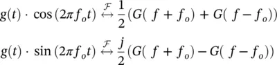
1.2.11 Derivation and Integration
If the derivative or integration of a time‐domain signal is taken, then the corresponding frequency‐domain signal is given as below.
(1.15) 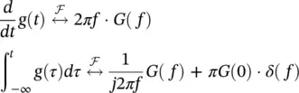
1.2.12 Parseval's Relationship
A useful property that was claimed by Parseval is that since the FT (or IFT) operation maps a signal in one domain to another domain, their energies should be exactly the same as given by the following relationship.
(1.16) 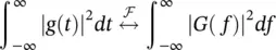
1.3 Time‐Frequency Representation of a Signal
While the FT concept can be successfully utilized for the stationary signals, there are many real‐world signals whose frequency contents vary over time. To be able to display these frequency variations over time; therefore, joint time–frequency (JTF) transforms/representations are being used.
1.3.1 Signal in the Time Domain
The term “time domain” is used while describing functions or physical signals with respect to time either continuous or discrete. The time‐domain signals are usually more comprehensible than the frequency‐domain signals since most of the real‐world signals are recorded and displayed versus time. Common equipment is to analyze time‐domain signals is the oscilloscope . In Figure 1.1, a time‐domain sound signal is shown. This signal is obtained by recording of an utterance of the word “prince” by a lady. By looking at the occurrence instants in the x ‐axis and the signal magnitude in the y ‐axis, one can analyze the stress of the letters inside the word “prince.”
1.3.2 Signal in the Frequency Domain
The term “frequency domain” is used while describing functions or physical signals with respect to frequency either continuous or discrete. Frequency‐domain representation has been proven to be very useful in innumerous engineering applications while characterizing, interpreting, and identifying signals. Solving differential equations, analyzing circuits, signal analysis in communication systems are few among many others where frequency‐domain representation is much more advantageous than the time‐domain representation. The frequency‐domain signal is traditionally obtained by taking the FT of the time‐domain signal. As briefly explained in Section 1.1, FT is generated by expressing the signal onto a set of basis functions, each of which is a sinusoid with the unique frequency. Displaying the measure of the similarities of the original time‐domain signal to those particular unique‐frequency bases generates the Fourier transformed signal or the frequency‐domain signal. Spectrum analyzers and network analyzers are the common equipments to analyze frequency‐domain signals. These signals are not as quite perceivable when compared to time‐domain signals. In Figure 1.2, the frequency‐domain version of the sound signal in Figure 1.1is obtained by using the DFT operation. The signal intensity value at each frequency component can be read from the y ‐axis. The frequency content of a signal is also called the spectrum of that signal.
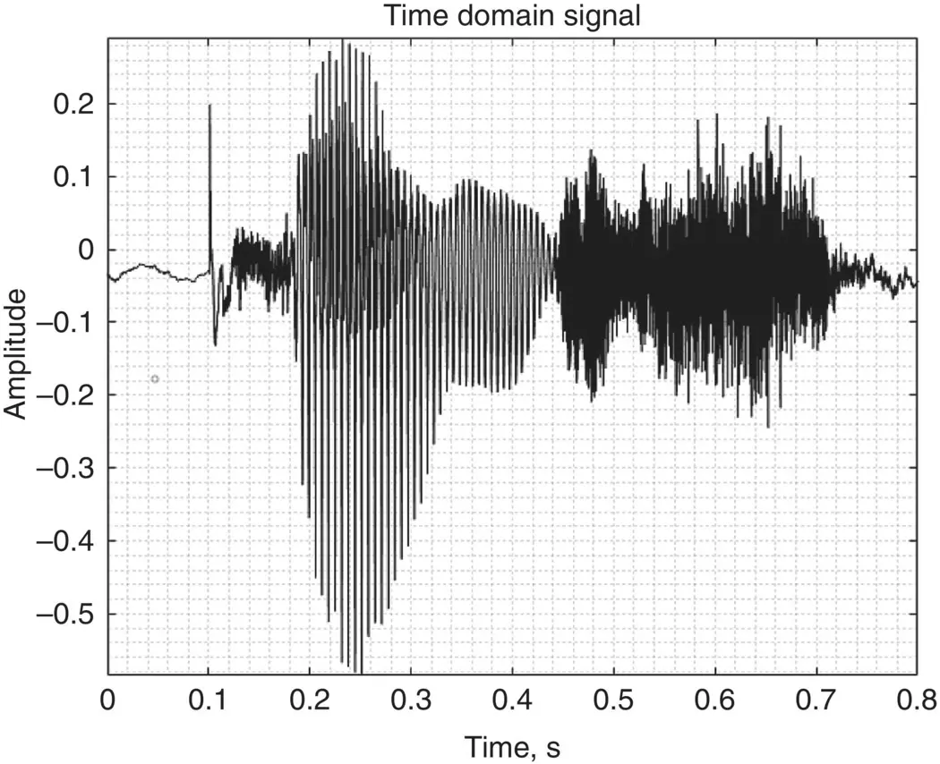
Figure 1.1 The time‐domain signal of “prince” spoken by a lady.
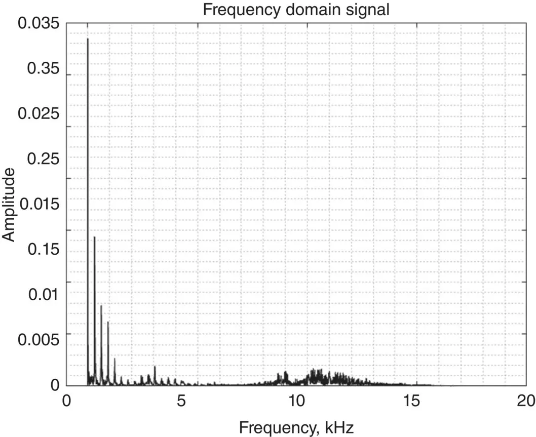
Figure 1.2 The frequency‐domain signal (or the spectrum) of “prince.”
1.3.3 Signal in the Joint Time‐Frequency (JTF) Plane
Although FT is very effective for demonstrating the frequency content of a signal, it does not give the knowledge of frequency variation over time. However, most of the real‐world signals have time‐varying frequency content such as speech and music signals. In these cases, the single‐frequency sinusoidal bases are not considered to be suitable for the detailed analysis of those signals. Therefore, JTF analysis methods were developed to represent these signals both in time and frequency to observe the variation of frequency content as the time progresses.
There are many tools to map a time domain or frequency‐domain signal onto the JFT plane. Some of the most well‐known JFT tools are short‐time Fourier transform (STFT) (Allen 1977), Wigner–Ville distribution (Nuttall 1988), Choi–Willams distribution (Du and Su 2003), Cohen's class (Cohen 1989), and time‐frequency distribution series (TFDS) (Qian and Chen 1996). Among these, the most appreciated and commonly used one is the STFT or the spectrogram . STFT can easily display the variations in the sinusoidal frequency and phase content of local moments of a signal over time with sufficient resolution in most cases.
The spectrogram transforms the signal onto two‐dimensional (2D) time‐frequency plane via the following famous equation:
(1.17) 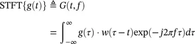
This transformation formula is nothing but the short‐time (or short‐term) version of the famous FT operation defined in Eq. 1.1. The main signal, g ( t ) is multiplied with a shorter duration window signal, w ( t ). By sliding this window signal over g ( t ) and taking the FT of the product, only the frequency content for the windowed version of the original signal is acquired. Therefore, after completing the sliding process over the whole duration of the time‐domain signal g ( t ) and putting corresponding FTs side by side, the 2D STFT of g ( t ) is obtained.
It is obvious that STFT will produce different output signals for different duration windows. The duration of the window affects the resolutions in both domains. While a very short‐duration time window provides a good resolution in the time direction, the resolution in the frequency direction becomes poor. This is because of the fact that the time duration and the frequency bandwidth of a signal are inversely proportional to each other. Similarly, a long duration time signal will give a good resolution in frequency domain while the resolution in the time domain will be bad. Therefore, a reasonable selection has to be bargained about the duration of the window in time to be able to view both domains with fairly good enough resolutions.
The shape of the window function has an effect on the resolutions as well. If a window with sharp ends is chosen, there will be strong side lobes in the other domain. Therefore, smooth waveform type windows are usually utilized to obtain well‐resolved images with less side lobes with the price of increased main beamwidth, i.e. less resolution. Commonly used window types are Hanning, Hamming, Kaiser, Blackman, and Gaussian.
Читать дальшеИнтервал:
Закладка:
Похожие книги на «Inverse Synthetic Aperture Radar Imaging With MATLAB Algorithms»
Представляем Вашему вниманию похожие книги на «Inverse Synthetic Aperture Radar Imaging With MATLAB Algorithms» списком для выбора. Мы отобрали схожую по названию и смыслу литературу в надежде предоставить читателям больше вариантов отыскать новые, интересные, ещё непрочитанные произведения.


Обсуждение, отзывы о книге «Inverse Synthetic Aperture Radar Imaging With MATLAB Algorithms» и просто собственные мнения читателей. Оставьте ваши комментарии, напишите, что Вы думаете о произведении, его смысле или главных героях. Укажите что конкретно понравилось, а что нет, и почему Вы так считаете.