Daniel J. Denis - Applied Univariate, Bivariate, and Multivariate Statistics
Здесь есть возможность читать онлайн «Daniel J. Denis - Applied Univariate, Bivariate, and Multivariate Statistics» — ознакомительный отрывок электронной книги совершенно бесплатно, а после прочтения отрывка купить полную версию. В некоторых случаях можно слушать аудио, скачать через торрент в формате fb2 и присутствует краткое содержание. Жанр: unrecognised, на английском языке. Описание произведения, (предисловие) а так же отзывы посетителей доступны на портале библиотеки ЛибКат.
- Название:Applied Univariate, Bivariate, and Multivariate Statistics
- Автор:
- Жанр:
- Год:неизвестен
- ISBN:нет данных
- Рейтинг книги:5 / 5. Голосов: 1
-
Избранное:Добавить в избранное
- Отзывы:
-
Ваша оценка:
Applied Univariate, Bivariate, and Multivariate Statistics: краткое содержание, описание и аннотация
Предлагаем к чтению аннотацию, описание, краткое содержание или предисловие (зависит от того, что написал сам автор книги «Applied Univariate, Bivariate, and Multivariate Statistics»). Если вы не нашли необходимую информацию о книге — напишите в комментариях, мы постараемся отыскать её.
contains an accessible introduction to statistical modeling techniques commonly used in the social and behavioral sciences. The text offers a blend of statistical theory and methodology and reviews both the technical and theoretical aspects of good data analysis.
Featuring applied resources at various levels, the book includes statistical techniques using software packages such as R and SPSS®. To promote a more in-depth interpretation of statistical techniques across the sciences, the book surveys some of the technical arguments underlying formulas and equations. The thoroughly updated edition includes new chapters on nonparametric statistics and multidimensional scaling, and expanded coverage of time series models. The second edition has been designed to be more approachable by minimizing theoretical or technical jargon and maximizing conceptual understanding with easy-to-apply software examples. This important text:
Offers demonstrations of statistical techniques using software packages such as R and SPSS® Contains examples of hypothetical and real data with statistical analyses Provides historical and philosophical insights into many of the techniques used in modern social science Includes a companion website that includes further instructional details, additional data sets, solutions to selected exercises, and multiple programming options Written for students of social and applied sciences,
offers a text to statistical modeling techniques used in social and behavioral sciences.
Applied Univariate, Bivariate, and Multivariate Statistics — читать онлайн ознакомительный отрывок
Ниже представлен текст книги, разбитый по страницам. Система сохранения места последней прочитанной страницы, позволяет с удобством читать онлайн бесплатно книгу «Applied Univariate, Bivariate, and Multivariate Statistics», без необходимости каждый раз заново искать на чём Вы остановились. Поставьте закладку, и сможете в любой момент перейти на страницу, на которой закончили чтение.
Интервал:
Закладка:
The null hypothesis is that the 50 counts making up the entire table are more or less randomly distributed across each of the cells. That is, there is no association between condition and exposure. We can easily test this hypothesis in SPSS by weighting the relevant frequencies by cell total:
| exposure | condition | freq |
| 1.00 | 0.00 | 10.00 |
| 1.00 | 1.00 | 20.00 |
| 2.00 | 0.00 | 15.00 |
| 2.00 | 1.00 | 5.00 |
WEIGHT BY freq. CROSSTABS /TABLES=condition BY exposure /FORMAT=AVALUE TABLES /STATISTICS=CHISQ /CELLS=COUNT /COUNT ROUND CELL.
The output follows in which it is first confirmed that we set up our data file correctly:
| Exposure * Condition Crosstabulation | ||||
|---|---|---|---|---|
| Count | ||||
| Condition | Total | |||
| 1.00 | 0.00 | |||
| Exposure | 1.00 | 20 | 10 | 30 |
| 2.00 | 5 | 15 | 20 | |
| Total | 25 | 25 | 50 |
We focus on the Pearson chi‐square test value of 8.3 on a single degree of freedom. It is statistically significant ( p = 0.004), and hence we can reject the null hypothesis of no association between condition and exposure group.
| Chi‐square Tests | |||||
| Value | d f | Asymp. Sig. (two‐sided) | Exact Sig. (two‐sided) | Exact Sig. (one‐sided) | |
| Pearson chi‐square | 8.333 a | 1 | 0.004 | ||
| Continuity correction b | 6.750 | 1 | 0.009 | ||
| Likelihood ratio | 8.630 | 1 | 0.003 | ||
| Fisher's exact test | 0.009 | 0.004 | |||
| Linear‐by‐linear association | 8.167 | 1 | 0.004 | ||
| No. of valid cases | 50 |
a 0 cells (0.0%) have expected count less than 5. The minimum expected count is 10.00.
b Computed only for a 2 × 2 table.
In R, we can easily perform the chi‐square test on this data. We first build the matrix of cell counts, calling it diag.table:
> diag.table <- matrix(c(20, 5, 10, 15), nrow = 2) > diag.table [,1] [,2] [1,] 20 10 [2,] 5 15 > chisq.test(diag.table, correct = F) Pearson's Chi-squared test data: diag.table X-squared = 8.3333, df = 1, p-value = 0.003892
We see that the result in R agrees with what we obtained in SPSS. Note that specifying correct = F(correction = false) negated what is known as Yates' correction for continuity, which involves subtracting 0.5 from positive differences in O − E and adding 0.5 to negative differences in O − E in an attempt to better make the chi‐square distribution approximate that of a multinomial distribution (i.e., in a crude sense, to help make discrete probabilities more continuous). To adjust for Yates, we can either specify correct = Tor simply chisq.test(diag.table), which will incorporate the correction. With the correction implemented, our p ‐value increases from 0.003 to 0.009 (not shown). We notice that this adjustment parallels that made in SPSS by adjusting for continuity. When expected counts per cell are relatively small (a working rule is that they should be at least five in each cell), one can also request Fisher' s exact test(see Fisher, 1922a), which we note also mirrors the output generated by SPSS:
> fisher.test(diag.table) Fisher's Exact Test for Count Data data: diag.table p-value = 0.008579 alternative hypothesis: true odds ratio is not equal to 1 95 percent confidence interval: 1.466377 26.597383 sample estimates: odds ratio 5.764989
Other useful statistics for contingency tables include the phi coefficientand Cramer's V. Phi, ϕ , is a measure of association for 2 × 2 contingency tables, computed as

where χ 2is the chi‐square statistic calculated on the 2 × 2 table, and n is the total sample size. The maximum ϕ can attain is 1.0, indicating maximal association. ϕ can be computed in SPSS by /statistics = phiand is available in R in the psychpackage (Revelle, 2015). Cramer's ϕ cextends on ϕ in that it allows for contingency tables of greater than 2 × 2. It is included in the /statistics = phicommand and also available in R's psychpackage. It is given by:
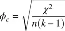
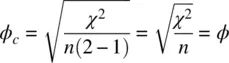
where k is the minimum of the number of rows or columns. The relationship between ϕ cand ϕ is easily shown for k = 2:
2.2.1 Power for Chi‐Square Test of Independence
We can estimate power 5 and required sample size for the chi‐square test of independence using the package pwrin R:
> library(pwr) > pwr.chisq.test (w =, N =, df =, sig.level =, power = )
where w is the anticipated or required effect size, estimated as:

and p 0 iand p 1 iare the probabilities in a given cell i under the null and alternative hypotheses, respectively. We demonstrate by estimating power for w = 0.2:
> pwr.chisq.test(w = 0.2, N =, df = 5, sig.level = .05, power = 0.90) Chi squared power calculation w = 0.2 N = 411.7366 df = 5 sig.level = 0.05 power = 0.9 NOTE: N is the number of observations
Table 2.2 Contingency Table for 2 × 2 × 2 Design
| Exposure | Condition Absent (0) | Condition Present (1) | Total | |
|---|---|---|---|---|
| Males | Yes | 10 | 20 | 30 |
| No | 15 | 5 | 20 | |
| Females | Yes | 13 | 17 | 30 |
| No | 12 | 8 | 20 | |
| Total | 50 | 50 | 100 |
R estimates that a total of approximately 411 subjects are required to achieve power set at 0.90. Such a large sample is required because w = 0.2 constitutes a relatively small effect size (see Cohen (1988) for details).
The reader may ask at this point how one might go about analyzing data for higher‐dimensional frequency tables. The example for the chi‐square test of the data in Table 2.1is only for that of a 2 × 2 layout. Suppose we added a third factor to our analysis, such as gender, making our contingency table appear as in Table 2.2.
For data such as that in Table 2.2featuring higher‐dimensional frequency data, log‐linear modelsare a possibility (Agresti, 2002). Log‐linear models are an option in the wider class of generalized linear models, to be discussed further in Chapter 10, where we discuss in some detail a special case of the generalized linear model called the logistic regression model.
Читать дальшеИнтервал:
Закладка:
Похожие книги на «Applied Univariate, Bivariate, and Multivariate Statistics»
Представляем Вашему вниманию похожие книги на «Applied Univariate, Bivariate, and Multivariate Statistics» списком для выбора. Мы отобрали схожую по названию и смыслу литературу в надежде предоставить читателям больше вариантов отыскать новые, интересные, ещё непрочитанные произведения.


Обсуждение, отзывы о книге «Applied Univariate, Bivariate, and Multivariate Statistics» и просто собственные мнения читателей. Оставьте ваши комментарии, напишите, что Вы думаете о произведении, его смысле или главных героях. Укажите что конкретно понравилось, а что нет, и почему Вы так считаете.