Daniel J. Denis - Applied Univariate, Bivariate, and Multivariate Statistics

> dbinom(5, size = 5, prob = 0.5) [1] 0.03125

Notice that the probability of obtaining five heads out of five flips on a fair coin is quite a bit less than that of obtaining two heads. We can continue to obtain the remaining probabilities and obtain the complete binomial distribution for this experiment:

A plot of this binomial distribution is given in Figure 2.4.

Suppose that instead of wanting to know the probability of getting two heads out of five flips, we wanted to know the probability of getting two or moreheads out of five flips. Because the events 2 heads, 3 heads, 4 heads, and 5 heads are mutually exclusive events, we can add their probabilities by the probability rule that says 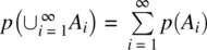: 0.3125 + 0.3125 + 0.15625 + 0.03125 = 0.8125. Hence, the probability of obtaining two or more heads on a fair coin on five flips is equal to 0.8125.

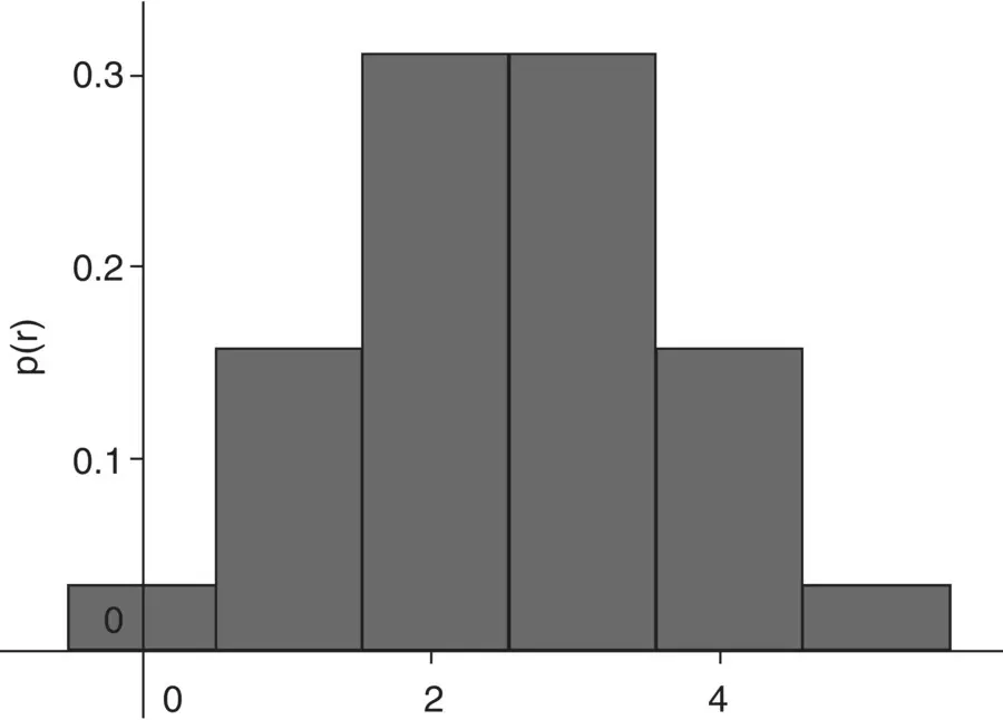
Figure 2.4Binomial distribution for the probability of the number of heads on a fair coin.

Binomial distributions are useful in a great variety of contexts in modeling a wide number of phenomena. But again, remember that the outcome of the variable must be binary, meaning it must have only twopossibilities. If it has more than two possibilities or is continuous in nature, then the binomial distribution is not suitable. Binomial data will be featured further in our discussion of logistic regression in Chapter 10.

One can also appreciate the general logic of hypothesis testing through the binomial. If our null hypothesis is that the coin is fair, and we obtain five heads out of five flips, this result has only a 0.03125 probability of occurring. Hence, because the probability of this data is so low under the model that the coin is fair, we typically decide to reject the null hypothesis and infer the statistical alternativehypothesis that p ( H ) ≠ 0.5. Substantively, we might infer that the coin is not fair, though this substantive alternativealso assumes it is the coin that is to “blame” for it coming up five times heads. If the flipper was responsible for biasing the coin, for instance, or a breeze suddenly came along that helped the result occur in this particular fashion, then inferring the substantive alternative hypothesis of “unfairness” may not be correct. Perhaps the natureof the coin is such that it isfair. Maybe the flipper or other factors (e.g., breeze) are what are ultimately responsible for the rejection of the null. This is one reason why rejecting null hypotheses is quite easy, but inferring the correctsubstantive alternative hypothesis (i.e., the hypothesis that explains whythe null was rejected) is much more challenging (see Denis, 2001). As concluded by Denis, “ Anyone can reject a null, to be sure. The real skill of the scientist is arriving at the true alternative.”

The binomial distribution is also well‐suited for comparing proportions. For details on how to run this simple test in R, see Crawley (2013, p. 365). One can also use binom.testin R to test simple binomial hypotheses, or the prop.testfor testing null hypotheses about proportions. A useful test that employs binomial distributions is the sign test(see Siegel and Castellan, 1988, pp. 80–87 for details). For a demonstration of the sign test in R, see Denis (2020).

Many distributions in statistics can be regarded as limiting formsof other distributions. What this statement means can be best demonstrated through an example of how the binomial and normal distributions are related. When the number of discrete categories along the x ‐axis grows larger and larger, the areas under the binomial distribution more and more resemble the probabilities computed under the normal curve. It is in this sense that for a large number of trials on the binomial, it begins to more closely approximatethe normal distribution.

As an example, consider once again the binomial distribution for n = 5, p = 0.5, but this time with a normal density overlaying the binomial ( Figure 2.5).

We can see that the normal curve “approximates” the binomial distribution, though perhaps not tremendously well for only five trials. If we increase the number of trials, however, to say, 20, the approximation is much improved. And when we increase the number of trials to 100, the binomial distribution looks virtually like a normal density. That is, we say that the normal distribution is the limiting form of the binomial distribution.

We can express this idea more formally. If the number of trials n in a binomial experiment is made large, the distribution of the number of successes x will tend to resemble a normal distribution. That is, the normal distribution is the limiting form of a binomial distribution as n → ∞ for a fixed p (and where q = 1 − p ), where E ( x i) is the expectation of the random variable x i(the meaning of “random variable” will be discussed shortly):

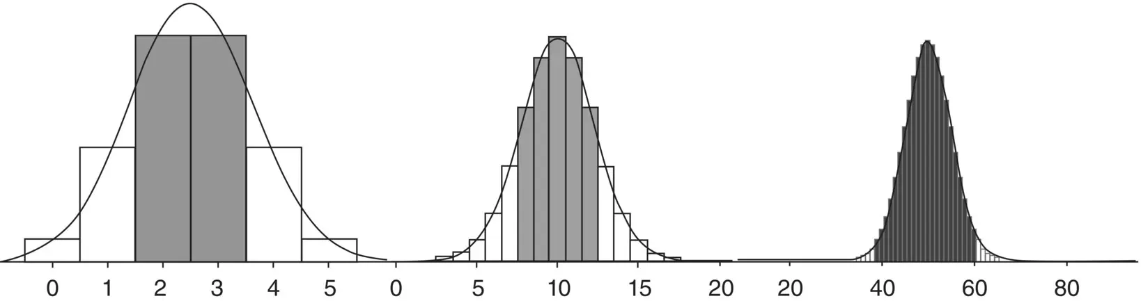
Figure 2.5Binomial distributions approximated by normal densities for 5 (far left), 20 (middle), and 100 trials (far right).

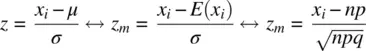
Notice that in a z ‐score calculation using the population mean μ , in the numerator, we are actually calculating the difference between the obtained score and the expectation, E ( x i). We can change this to a binomial function by replacing the expectation μ with the expectation from a binomial distribution, that is, np , where np is the mean of a binomial distribution. Similarly, we replace the standard deviation from a normal distribution with the standard deviation from the binomial distribution, . As n grows infinitely large, the normal and the binomial probabilities become identical for any standardized interval. 3

A univariate density expresses the probability of a single random variable within a specified interval of values along the abscissa. A joint probability density, analogous to a joint probability, expresses the probability of simultaneously observing tworandom variables over a given interval of values. The bivariate normal densityis given by:

where ρ 2is the squared Pearson correlation coefficient between x 1and x 2.