Daniel J. Denis - Applied Univariate, Bivariate, and Multivariate Statistics

In spite of the immense amount of fruitful labour which has been expended in its practical applications, the basic principles of this organ of science are still in a state of obscurity, and it cannot be denied that, during the recent rapid development of practical methods, fundamental problems have been ignored and fundamental paradoxes left unresolved.

(Fisher, 1922a, p. 310)

Our statistics review includes topics that would customarily be seen in a first course in statistics at the undergraduate level, but depending on the given course and what was emphasized by the instructor, our treatment here may be at a slightly deeper level. We review these principles with demonstrations in R and SPSS where appropriate. Should any of the following material come across as entirely “new,” then a review of any introductory statistics text is recommended. For instance, Kirk (2008), Moore, McCabe, and Craig (2014), Box, Hunter, and Hunter (1978) are relatively nontechnical sources, whereas Degroot and Schervish (2002), Wackerly, Mendenhall III, and Scheaffer (2002) along with Evans and Rosenthal (2010) are much deeper and technically dense. Casella and Berger (2002), Hogg and Craig (1995) along with Shao (2003) are much higher‐level theoretically oriented texts targeted mainly at mathematical and theoretical statisticians. Other sources include Panik (2005), Berry and Lindgren (1996), and Rice (2006). For a lighter narrative on the role of statistics in social science, consult Abelson (1995).

Because of its importance in the interpretation of evidence, we close the chapter with an easy but powerful demonstration of what makes a p ‐value small or large in the context of statistical significance testing and the testing of null hypotheses. It is imperative that as a research scientist, you are knowledgeable of this material before you attempt to evaluate anyresearch findings that employ statistical inference.

When we speak of densityas it relates to distributions in statistics, we are referring generally to theoretical distributions having area under their curves. There are numerous probability distributions or density functions. Empirical distributions, on the other hand, rarely go by the name of densities. They are in contrast “real” distributions of real empirical data. In some contexts, the identifier normal distributionmay be given without reference as to whether one is referring to a density or to an empirical distribution. It is usually evident by the context of the situation which we are referring to. We survey only a few of the more popular densities and distributions in our discussion that follows.

The univariate normal density is given by:

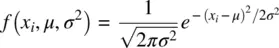
where,

μ is the population mean for the given density,

σ2 is the population variance,

π is a constant equal to approximately 3.14,

e is a constant equal to approximately 2.71,

xi is a given value of the independent variable, assumed to be a real number.

When μ is 0 and σ 2is 1, which implies that the standard deviation σ is also equal to 1 (i.e., 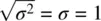), the normal distribution is given a special name. It is called the standard normal distributionand can be written more compactly as:

(2.1)

Notice that in (2.1), 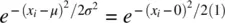where μ is now 0 and σ 2is now 1. Note as well that the density depends only on the absolutevalue of x i, because both x iand − x igive the same value ; the greater is x iin absolute value, the smaller the density at that point, because the constant e is raised to the negativepower .

The standard normal distributionis the classic z ‐distribution whose areas under the curve are given in the appendices of most statistics texts, and are more conveniently computed by software. An example of the standard normal is featured in Figure 2.1.

Scores in research often come in their own units, with distributions having means and variances different from 0 and 1. We can transform a score coming from a given distribution with mean μ and standard deviation σ by the familiar z ‐score:

A z ‐score is expressed in units of the standard normal distribution. For example, a z ‐score of +1 denotes that the given raw score lay one standard deviation above the mean. A z ‐score of −1 means that the given raw score lay one standard deviation below the mean. In some settings (such as school psychology), t ‐scores are also useful, having a mean of 50 and standard deviation of 10. In most contexts, however, z ‐scores dominate.

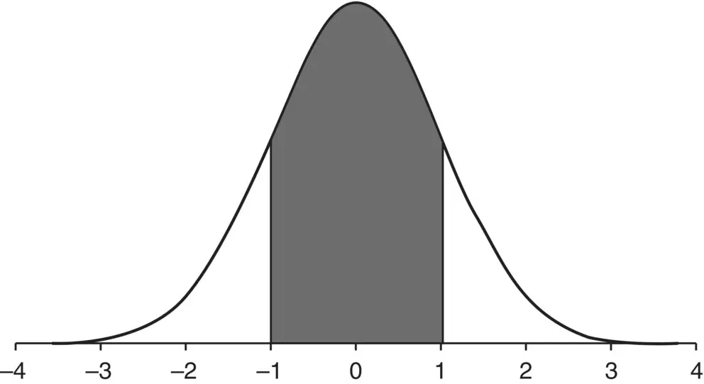
Figure 2.1Standard normal distribution with shaded area from −1 to +1 standard deviations from the mean.

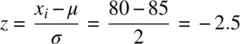
A classic example of the utility of z ‐scores typically goes like this. Suppose two sections of a statistics course are being taught. John is a student in section A and Mary is a student in section B. On the final exam for the course, John receives a raw score of 80 out of 100 (i.e., 80%). Mary, on the other hand, earns a score of 70 out of 100 (i.e., 70%). At first glance, it may appear that John was more successful on his final exam. However, scores, considered absolutely, do not allow us a comparison of each student's score relative to their class distributions. For instance, if the mean in John's class was equal to 85% with a standard deviation of 2, this means that John's z ‐score is:

Suppose that in Mary's class, the mean was equal to 65% also with a standard deviation of 2. Mary's z ‐score is thus:

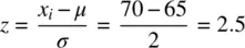
As we can see, relative to their particular distributions, Mary greatly outperformed John. Assuming each distribution is approximately normal, the density under the curve for a normal distribution with mean 0 and standard deviation of 1 at a score of 2.5 is: