John E. Boylan - Intermittent Demand Forecasting
Здесь есть возможность читать онлайн «John E. Boylan - Intermittent Demand Forecasting» — ознакомительный отрывок электронной книги совершенно бесплатно, а после прочтения отрывка купить полную версию. В некоторых случаях можно слушать аудио, скачать через торрент в формате fb2 и присутствует краткое содержание. Жанр: unrecognised, на английском языке. Описание произведения, (предисловие) а так же отзывы посетителей доступны на портале библиотеки ЛибКат.
- Название:Intermittent Demand Forecasting
- Автор:
- Жанр:
- Год:неизвестен
- ISBN:нет данных
- Рейтинг книги:5 / 5. Голосов: 1
-
Избранное:Добавить в избранное
- Отзывы:
-
Ваша оценка:
Intermittent Demand Forecasting: краткое содержание, описание и аннотация
Предлагаем к чтению аннотацию, описание, краткое содержание или предисловие (зависит от того, что написал сам автор книги «Intermittent Demand Forecasting»). Если вы не нашли необходимую информацию о книге — напишите в комментариях, мы постараемся отыскать её.
The first text to focus on the methods and approaches of intermittent, rather than fast, demand forecasting
Intermittent Demand Forecasting No prior knowledge of intermittent demand forecasting or inventory management is assumed in this book. The key formulae are accompanied by worked examples to show how they can be implemented in practice. For those wishing to understand the theory in more depth, technical notes are provided at the end of each chapter, as well as an extensive and up-to-date collection of references for further study. Software developments are reviewed, to give an appreciation of the current state of the art in commercial and open source software.
“Intermittent demand forecasting may seem like a specialized area but actually is at the center of sustainability efforts to consume less and to waste less. Boylan and Syntetos have done a superb job in showing how improvements in inventory management are pivotal in achieving this. Their book covers both the theory and practice of intermittent demand forecasting and my prediction is that it will fast become the bible of the field.” —
, Professor, University of Nicosia, and Director, Institute for the Future and the Makridakis Open Forecasting Center (MOFC).
“We have been able to support our clients by adopting many of the ideas discussed in this excellent book, and implementing them in our software. I am sure that these ideas will be equally helpful for other supply chain software vendors and for companies wanting to update and upgrade their capabilities in forecasting and inventory management.”—
, VP, Research and Development, Blue Yonder.
“As product variants proliferate and the pace of business quickens, more and more items have intermittent demand. Boylan and Syntetos have long been leaders in extending forecasting and inventory methods to accommodate this new reality. Their book gathers and clarifies decades of research in this area, and explains how practitioners can exploit this knowledge to make their operations more efficient and effective.”—
, Professor Emeritus, Rensselaer Polytechnic Institute.
Intermittent Demand Forecasting — читать онлайн ознакомительный отрывок
Ниже представлен текст книги, разбитый по страницам. Система сохранения места последней прочитанной страницы, позволяет с удобством читать онлайн бесплатно книгу «Intermittent Demand Forecasting», без необходимости каждый раз заново искать на чём Вы остановились. Поставьте закладку, и сможете в любой момент перейти на страницу, на которой закончили чтение.
Интервал:
Закладка:
In our example, the calculations were manageable because the protection interval was only for two periods and the OUT level did not need to exceed four units. The calculations can become more involved for longer protection intervals and higher OUT levels, and approximate formulae have been given to simplify the calculations (Cardós and Babiloni 2011). In Chapter 8, we explain how other formulae can be used if the demand follows certain demand distributions. If no demand distributions can adequately represent the real demand, then another option is to use non‐parametric approaches, to be discussed in Chapter 13.
3.5.4 Summary
There are two approaches to measuring the cycle service level. These methods produce the same results for non‐intermittent demand. They differ for intermittent items because the second method excludes those cycles with no demand during the review interval. This makes more sense for intermittence, but it complicates the calculation, which depends on combining two different demand distributions, one for the review interval and one for the lead time.
3.6 Calculating Fill Rates
The unit fill rate is defined as the proportion of demand satisfied directly from stock on hand, as noted earlier. It can be calculated at both aggregate and SKU levels, and can be defined in terms of volume filled or value filled. At SKU level, volume and value fill rates will be the same (unless calculated over a period of time in which there has been a price change) but will usually differ at an aggregate level. In this section, we look at some of the issues that need to be addressed in finding the unit (volume) fill rate, and discuss how demand distributions can be used in its calculation.
3.6.1 Unit Fill Rates
The basic unit fill rate calculation is straightforward. For example, if in a particular period we satisfy three units out of four demanded directly from stock, then the fill rate is 75%. Let us now consider an example of four periods with each period showing some demand, as shown in Table 3.6.
How should we define the overall fill rate? There are two possible approaches. The first is to total the satisfied demand (8 units) and divide by the total demand (16 units) to give an overall fill rate of 50%, as shown in Table 3.6. The second approach is to average the fill rates over all four periods, giving an overall fill rate of 56.25%, which is somewhat higher than the first calculation. If all four periods had a fill rate of 50%, then the two calculation methods would agree. The disagreement arises because the average of the fill rates in the second and third periods is 62.5%, whereas only 50% of the total demand over these two periods is fulfilled. The second method can be applied to intermittent demand only if periods with zero demands are excluded from the calculation. For further discussion of this method, please refer to Guijarro et al. (2012). We will base our analysis on the first method, as it is simpler for intermittent demand, and is the standard method in the literature and in practice.
Table 3.6 Fill rates per time period.
| Period | Demand | Satisfied | Fill rate |
|---|---|---|---|
| 1 | 2 | 1 | 0.50 |
| 2 | 4 | 1 | 0.25 |
| 3 | 2 | 2 | 1.00 |
| 4 | 8 | 4 | 0.50 |
| Total | 16 | 8 | 0.50 |
3.6.2 Fill Rates: Standard Formula
To calculate the unit fill rate (FR), we need to evaluate how much demand is satisfied, over a given period of time, as a proportion of the demand over the same period. Equivalently, we can evaluate the average unsatisfied demand per period, as a proportion of the average demand per period, and subtract this ratio from one, as shown in Eq. (3.2).
(3.2) 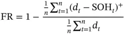
where  represents the stock on hand at the start of time period
  , after receipt of any orders and dispatch of any outstanding backorders,
  is demand during time period
  , and
, and  is the number of time periods over which the fill rate is being measured. The superscript
  indicates a result of zero if the expression in the brackets is negative, and unchanged otherwise. For example,
  and
and  .
.
In Eq. (3.2), the expression 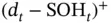 represents the backorders generated at the end of period
  as a consequence of demand in that period not being satisfied. If there is sufficient stock (
  less than or equal to
  ), then there are no backorders. If there is insufficient stock (
  strictly greater than
  ), then
  units are backordered. In the numerator of the ratio in Eq. (3.2), the backorders are summed over all periods and divided by the number of periods (
  ) to give the average unsatisfied demand per period. In the denominator, we have the average demand per period. The ratio represents the average unsatisfied demand per period as a proportion of the average demand per period.
For ease of exposition, from this point on, we assume that the review interval is one period (  ). At the end of this section, we return to the more general case when it can be longer.
Интервал:
Закладка:
Похожие книги на «Intermittent Demand Forecasting»
Представляем Вашему вниманию похожие книги на «Intermittent Demand Forecasting» списком для выбора. Мы отобрали схожую по названию и смыслу литературу в надежде предоставить читателям больше вариантов отыскать новые, интересные, ещё непрочитанные произведения.


Обсуждение, отзывы о книге «Intermittent Demand Forecasting» и просто собственные мнения читателей. Оставьте ваши комментарии, напишите, что Вы думаете о произведении, его смысле или главных героях. Укажите что конкретно понравилось, а что нет, и почему Вы так считаете.