Anand K. Verma - Introduction To Modern Planar Transmission Lines
Здесь есть возможность читать онлайн «Anand K. Verma - Introduction To Modern Planar Transmission Lines» — ознакомительный отрывок электронной книги совершенно бесплатно, а после прочтения отрывка купить полную версию. В некоторых случаях можно слушать аудио, скачать через торрент в формате fb2 и присутствует краткое содержание. Жанр: unrecognised, на английском языке. Описание произведения, (предисловие) а так же отзывы посетителей доступны на портале библиотеки ЛибКат.
- Название:Introduction To Modern Planar Transmission Lines
- Автор:
- Жанр:
- Год:неизвестен
- ISBN:нет данных
- Рейтинг книги:4 / 5. Голосов: 1
-
Избранное:Добавить в избранное
- Отзывы:
-
Ваша оценка:
Introduction To Modern Planar Transmission Lines: краткое содержание, описание и аннотация
Предлагаем к чтению аннотацию, описание, краткое содержание или предисловие (зависит от того, что написал сам автор книги «Introduction To Modern Planar Transmission Lines»). Если вы не нашли необходимую информацию о книге — напишите в комментариях, мы постараемся отыскать её.
rovides a comprehensive discussion of planar transmission lines and their applications, focusing on physical understanding, analytical approach, and circuit models
Planar transmission lines form the core of the modern high-frequency communication, computer, and other related technology. This advanced text gives a complete overview of the technology and acts as a comprehensive tool for radio frequency (RF) engineers that reflects a linear discussion of the subject from fundamentals to more complex arguments.
Introduction to Modern Planar Transmission Lines: Physical, Analytical, and Circuit Models Approach Emphasizes modeling using physical concepts, circuit-models, closed-form expressions, and full derivation of a large number of expressions Explains advanced mathematical treatment, such as the variation method, conformal mapping method, and SDA Connects each section of the text with forward and backward cross-referencing to aid in personalized self-study
is an ideal book for senior undergraduate and graduate students of the subject. It will also appeal to new researchers with the inter-disciplinary background, as well as to engineers and professionals in industries utilizing RF/microwave technologies.
Introduction To Modern Planar Transmission Lines — читать онлайн ознакомительный отрывок
Ниже представлен текст книги, разбитый по страницам. Система сохранения места последней прочитанной страницы, позволяет с удобством читать онлайн бесплатно книгу «Introduction To Modern Planar Transmission Lines», без необходимости каждый раз заново искать на чём Вы остановились. Поставьте закладку, и сможете в любой момент перейти на страницу, на которой закончили чтение.
Интервал:
Закладка:
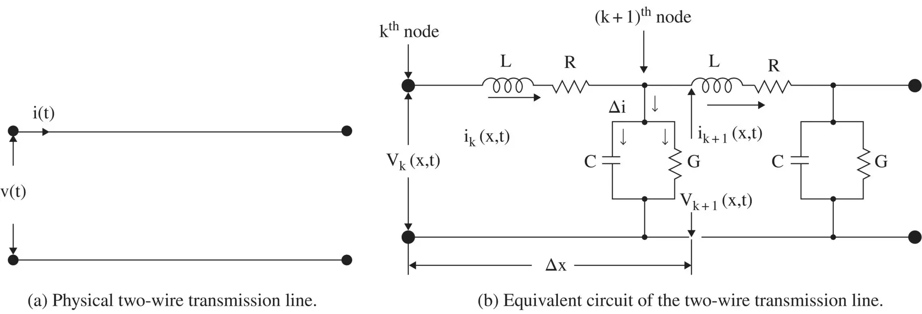
Figure 2.6 RLCG lumped circuit model of a transmission line.
A two‐conductor transmission line, or any other line supporting the TEM mode, is modeled as a chain of discrete passive RLCG components. As a matter of fact, by cascading several sections of discrete L‐network of the series L and shunt C elements, or even discrete L‐network of the series C and shunt L elements, an artificial transmission line can also be constructed. The artificial transmission line is discussed in section (3.4)of chapter 3, and also in the chapters 19and 22. It plays a very important role in modern microwave planar technology. The behavior of a transmission line is determined in terms of the resistor (R), inductor (L), capacitor (C), and conductance (G); all line elements are in per unit length, i.e. p.u.l . Kelvin introduced the modeling of the telegraph cable laid in the ocean using the RC circuit model . Heaviside further introduced L and G components in the circuit model to improve the modeling of the lossy transmission line [B.1, B.2, J.1, J.2]. Kelvin RC‐circuit model of the transmission line leads to the diffusion equation, not to the wave equation. Whereas using the RLGC circuit model, Heaviside finally obtained the wave equation for the voltage/current on a transmission line. Using the RLCG circuit model, shown in Fig (2.6b), the voltage, and current equations are obtained for the transmission line. The set of the coupled voltage and current equations are normally called the telegrapher's equations; as it was originally developed for the telegraph cables. However, the set of coupled transmission line equations can be called the Kelvin–Heaviside transmission line equations to recognize their contributions.
The Resistance of a Line
The electrical loss in a transmission line, known as the conductor loss , is due to the finite conductivity of the line. It is modeled as the resistance R p.u.l . It is also influenced by the skin effect phenomena at a higher frequency. The instantaneous current i ( t ) flowing through a lumped resistance R lumis related to the instantaneous voltage drop v ( t ) by Ohm's law:
(2.1.12) 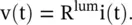
The Inductance of a Line
The current flowing in a conductor creates the magnetic field around itself. So the magnetic energy stored in the space around the transmission line, i.e. the time‐varying current supporting line section, is modeled by a series inductor L p.u.l . The inductance of a line is not lumped at one point, i.e. it is not confined at one point. It is distributed over the whole length of a line. The instantaneous voltage across a lumped inductor L lumis related to the current flowing through it by
(2.1.13) 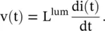
The Capacitance of a Line
In a two‐conductor transmission line, the conductors separated by a dielectric medium form a distributed system of capacitance. The electric field energy stored in a line is modeled by the shunt capacitance C p.u.l . The instantaneous shunt current through a lumped capacitor C lumis related to the instantaneous voltage across it by
(2.1.14) 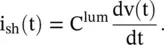
The Conductance of a Line
If the medium between two conductors of the transmission line is not a perfect dielectric, i.e. if it has finite conductivity, then a part of the line current shunts through the medium causing the dielectric loss . The dielectric loss of the line is modeled by shunt conductance G p.u.l . The instantaneous shunt current is related to the instantaneous voltage across a lumped conductance by
(2.1.15) 
Figure (2.6a)shows a physical transmission line that supports the TEM mode wave propagation. Figure (2.6b)shows that this line could be modeled as a chain of the lumped RLCG structure. More numbers of RLCG sections per wavelength are needed to model a transmission line. The RLCG model is the modeling of a transmission line by the lossy series inductor and lossy shunt capacitor. The transmission line supports the wave propagation from power AC to RF and above. Likewise, the corresponding lumped components model of a transmission line also supports such waves. The transmission line structure behaves like a low‐pass filter.
2.1.3 Kelvin–Heaviside Transmission Line Equations in Time Domain
Figure (2.6b)shows the lumped element equivalent circuit model of a section Δx of the transmission line. The primary line constants R, L, C, G on the per unit length ( p.u.l .) basis are related to the lumped circuit elements as R lum= RΔx, L lum= LΔx, C lum= CΔx, and G lum= GΔx. Figure (2.6b)shows the voltage loop equation and the current node equation for a small line section Δx. These are written as follows:
The Loop Equation
Differential voltage change across line length Δx = Voltage drop across inductor + Voltage drop across resistance
(2.1.16) 
The instantaneous line voltage v(t) and the instantaneous line current i(t) are functions of the space–time variables x and t. In the limiting case of Δx → 0, equation (2.1.16)is written as
(2.1.17) 
The Node Equation
Differential shunt current at the node = Current through conductance + Current through capacitor
(2.1.18) 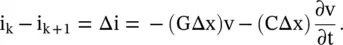
In the limiting case, Δx → 0; and the above equation is written as
(2.1.19) 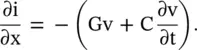
The pair of coupled voltage and current transmission line equations in the time‐domain summarized below is known as “ the time domain telegrapher's equations ”:
(2.1.20) 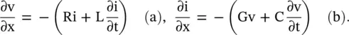
The above pair of equations can also be called the Kelvin–Heaviside transmission line equations . The coupled Kelvin–Heaviside transmission line equations relate the voltage and current on a transmission line through the line parameters, RLCG. These parameters are known as the primary constants of a line. The RLCG parameters depend on the physical configuration of a line, i.e. on its physical shapes, dimensions, and the electrical properties of the medium. They could be frequency‐dependent parameters also. For simple transmission lines such as a pair of wires and coaxial lines, the closed‐form formulas are available to compute them. However, these parameters could also be obtained through measurements. The empirical expressions for the RLCG parameters of a microstrip line are also available [J.3]. The transmission line equations are the complementary parts of Maxwell's field equations that relate the time‐varying electric and magnetic fields in a physical medium through the primary constants of a medium‐conductivity (σ), permittivity (ε) and permeability (μ). It is discussed in chapter 4. The transmission line equations can be obtained from Maxwell's equations. It is discussed in section (7.3) of chapter 7.
Читать дальшеИнтервал:
Закладка:
Похожие книги на «Introduction To Modern Planar Transmission Lines»
Представляем Вашему вниманию похожие книги на «Introduction To Modern Planar Transmission Lines» списком для выбора. Мы отобрали схожую по названию и смыслу литературу в надежде предоставить читателям больше вариантов отыскать новые, интересные, ещё непрочитанные произведения.


Обсуждение, отзывы о книге «Introduction To Modern Planar Transmission Lines» и просто собственные мнения читателей. Оставьте ваши комментарии, напишите, что Вы думаете о произведении, его смысле или главных героях. Укажите что конкретно понравилось, а что нет, и почему Вы так считаете.