Anand K. Verma - Introduction To Modern Planar Transmission Lines

(2.1.4)

In equation (2.1.4), the lagging phase ϕ = βx is caused by the delay in oscillation at the receiving end. The medium supporting the wave motion is assumed to be lossless. The wave variable v(t, x) is a doubly periodic function of both time and space coordinates as shown in Fig (2.2a and b), respectively.

The temporal period, i.e. time‐period T is related to the angular frequency ω as follows:

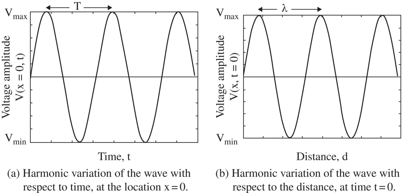
Figure 2.2 Double periodic variations of wave motion.

(2.1.5)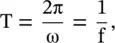

where f is the frequency in Hz (Hertz), i.e. the number of cycles per sec. The wavelength (λ) describes the spatial period , i.e. space periodicity. It is related to the phase‐shift constant (or phase constant) , i.e. the propagation constant β, as follows:

(2.1.6)

The wave motion or velocity of a monochromatic wave (the wave of a single frequency) is the motion of its wavefront . For the 3D wave motion in an isotropic space, the wavefront is a surface of the constant phase. In the case of the 1D wave motion, the wavefront is a line, whereas, for the 2D wave motion on an isotropic surface, the wavefront is a circle.

Figure (2.3)shows the peak point P at the wavefront of the ID wave. The motion of a constant phase surface is known as its phase velocity v p. Thus, the peak point P at the wavefront has moved to a new location P ′in such a way that phase of the propagating wave remains constant, i.e. ωt − βx = constant. On differentiating the constant phase with respect to time t, the expression for the phase velocity is obtained:

Figure 2.3 Wave motion as a motion of constant phase surface. It is shown as the moving point P.

(2.1.7)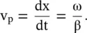

In a nondispersive medium, the phase velocity of a wave is independent of frequency, i.e. the waves of all frequencies travel at the same velocity. Figure (2.4)shows the nondispersive wave motion on the (ω − β) diagram. It is a linear graph . The slope of the point Q on the dispersion diagram subtends an angle θ at the origin that corresponds to the phase velocity of a propagating wave,

(2.1.8)

Thus, for a frequency‐independent nondispersive wave, the phase constant is a linear function of angular frequency.

(2.1.9)

The dispersive nature of the 1D wave motion is further discussed in sections ( 3.3) and ( 3.4) of the chapter 3. The phase velocity in a dispersive medium is usually frequency‐dependent. It is known as the temporal dispersion . In some cases, the phase velocity could also depend on wavevector (β, or k). It is known as spatial dispersion . The spatial dispersion is discussed in the subsection (21.1.1) of the chapter 21. The dispersion diagrams of the wave propagation in the isotropic and anisotropic media are further discussed in the section (4.7)of the chapter 4, and also in the section (5.2)of chapter 5.

Figure 2.4 The ω‐β dispersion diagram of nondispersive wave.

The one‐dimensional (1D) wave travels both in the forward and in the backward directions. It can have any arbitrary shape. In general, the 1D wave propagation can be described by the following wave function , known as the general wave equation :

(2.1.10)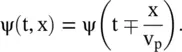

On taking the second‐order partial derivative of the wave function ψ(t, x) with respect to space‐time coordinate x and t, the 1D second‐order partial differential equation (PDE) of the wave equation is obtained. Similarly, wave functions ψ(t, x, y) and ψ(t, x, y, z) are solutions of two‐dimensional (2D) and three‐dimensional (3D) wave equations supported by the surface and free space medium, respectively. These PDEs are summarized below:

(2.1.11)

The dispersion diagram of the 2D wave propagation over the (x, y) surface is obtained by revolving the slant line of Fig (2.4)around the ω‐axis with propagation constants β x, β yin the x ‐ and y ‐direction. It is discussed in subsection ( 4.7.4) of chapter 4.

A physical transmission line, supporting the voltage/current wave, can be modeled by the lumped R, L, C, G components, i.e. the resistance, inductance, capacitance, and conductance per unit length ( p.u.l .), respectively. The two‐conductor transmission line can acquire many physical forms. A few of these forms are shown in Fig (2.5). The lines as shown in Fig (2.5a–c)support the wave propagation in the transverse electro magnetic mode, i.e. in the TEM‐mode; while Fig ( 2.5 c) shows the quasi‐TEM mode‐supporting microstrip . For TEM mode wave propagation, the electric field and magnetic field are normal to each other and also normal to the direction of wave propagation. For the TEM mode, there is no field component along the direction of propagation. However, the quasi‐TEM mode also has component of weak fields along the longitudinal direction of wave propagation. The quasi‐TEM mode is a hybrid mode discussed in the subsection (7.1.4) of chapter 7.

All TEM mode supporting transmission lines can be represented by a parallel two‐wire transmission line shown in Fig (2.6a). A transmission line is a 1D wave supporting structure. Its cross‐sectional dimension is much less than λ/4; otherwise, its TEM nature is changed. The longitudinal dimension can have any value, from a fraction of a wavelength to several wavelengths. The mode theory of the electromagnetic (EM) wave propagation is further discussed in chapter 7.

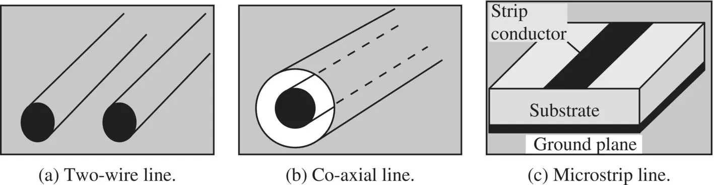
Figure 2.5 Cross‐section of a few two‐conductor transmission lines.