Ernest P. Chan - Quantitative Trading

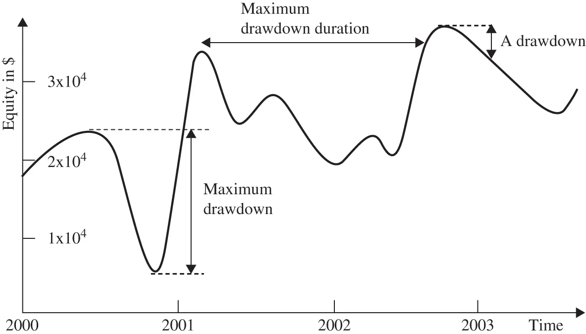
FIGURE 2.1Drawdown, maximum drawdown, and maximum drawdown duration.

As a rule of thumb, any strategy that has a Sharpe ratio of less than 1 is not suitable as a stand-alone strategy. For a strategy that achieves profitability almost every month, its (annualized) Sharpe ratio is typically greater than 2. For a strategy that is profitable almost every day, its Sharpe ratio is usually greater than 3. I will show you how to calculate Sharpe ratios for various strategies in Examples 3.4, 3.6, and 3.7in the next chapter.

A strategy suffers a drawdown whenever it has lost money recently. A drawdown at a given time t is defined as the difference between the current equity value (assuming no redemption or cash infusion) of the portfolio and the global maximum of the equity curve occurring on or before time t . The maximum drawdown is the difference between the global maximum of the equity curve with the global minimum of the curve after the occurrence of the global maximum (time order matters here: The global minimum must occur later than the global maximum). The global maximum is called the high watermark . The maximum drawdown duration is the longest it has taken for the equity curve to recover losses.

More often, drawdowns are measured in percentage terms, with the denominator being the equity at the high watermark and the numerator being the loss of equity since reaching the high watermark.

Figure 2.1illustrates a typical drawdown, the maximum drawdown, and the maximum drawdown duration of an equity curve. I will include a tutorial in Example 3.5 on how to compute these quantities from a table of daily profits and losses using either Excel, MATLAB, Python, or R. One thing to keep in mind: The maximum drawdown and the maximum drawdown duration do not typically overlap over the same period.

Defined mathematically, drawdown seems abstract and remote. However, in real life there is nothing more gut-wrenching and emotionally disturbing to suffer than a drawdown if you're a trader. (This is as true for independent traders as for institutional ones. When an institutional trading group is suffering a drawdown, everybody seems to feel that life has lost meaning and spend their days dreading the eventual shutdown of the strategy or maybe even the group as a whole.) It is therefore something we would want to minimize. You have to ask yourself, realistically, how deep and how long a drawdown will you be able to tolerate and not liquidate your portfolio and shut down your strategy? Would it be 20 percent and three months, or 10 percent and one month? Comparing your tolerance with the numbers obtained from the backtest of a candidate strategy determines whether that strategy is for you.

Even if the author of the strategy you read about did not publish the precise numbers for drawdowns, you should still be able to make an estimate from a graph of its equity curve. For example, in Figure 2.1, you can see that the longest drawdown goes from around February 2001 to around October 2002. So the maximum drawdown duration is about 20 months. Also, at the beginning of the maximum drawdown, the equity was about $2.3 × 10 4, and at the end, about $0.5 × 10 4. So the maximum drawdown is about $1.8 × 10 4.

Every time a strategy buys and sells a security, it incurs a transaction cost. The more frequently it trades, the larger the impact of transaction costs will be on the profitability of the strategy. These transaction costs are not just due to commission fees charged by the broker. There will also be the cost of liquidity—when you buy and sell securities at their market prices, you are paying the bid–ask spread. If you buy and sell securities using limit orders, however, you avoid the liquidity costs but incur opportunity costs. This is because your limit orders may not be executed, and therefore you may miss out on the potential profits of your trade. Also, when you buy or sell a large chunk of securities, you will not be able to complete the transaction without impacting the prices at which this transaction is done. (Sometimes just displaying a bid to buy a large number of shares for a stock can move the prices higher without your having bought a single share yet!) This effect on the market prices due to your own order is called market impact, and it can contribute to a large part of the total transaction cost when the security is not very liquid.

Finally, there can be a delay between the time your program transmits an order to your brokerage and the time it is executed at the exchange, due to delays on the internet or various software-related issues. This delay can cause a slippage, the difference between the price that triggers the order and the execution price. Of course, this slippage can be of either sign, but on average it will be a cost rather than a gain to the trader. (If you find that it is a gain on average, you should change your program to deliberately delay the transmission of the order by a few seconds!)

Transaction costs vary widely for different kinds of securities. You can typically estimate it by taking half the average bid–ask spread of a security and then adding the commission if your order size is not much bigger than the average sizes of the best bid and offer. If you are trading S&P 500 stocks, for example, the average transaction cost (excluding commissions, which depend on your brokerage) would be about 5 basis points (that is, five-hundredths of a percent). Note that I count a round-trip transaction of a buy and then a sell as two transactions—hence, a round trip will cost 10 basis points in this example. If you are trading ES, the E-mini S&P 500 futures, the transaction cost will be about 1 basis point. Sometimes the authors whose strategies you read about will disclose that they have included transaction costs in their backtest performance, but more often they will not. If they haven't, then you just to have to assume that the results are before transactions, and apply your own judgment to its validity.

As an example of the impact of transaction costs on a strategy, consider this simple mean-reverting strategy on ES. It is based on Bollinger Bands: that is, every time the price exceeds plus or minus 2 moving standard deviations of its moving average, short or buy, respectively. Exit the position when the price reverts back to within 1 moving standard deviation of the moving average. If you allow yourself to enter and exit every five minutes, you will find that the Sharpe ratio is about 3 without transaction costs—very excellent indeed! Unfortunately, the Sharpe ratio is reduced to –3 if we subtract 1 basis point as transaction costs, making it a very unprofitable strategy.

For another example of the impact of transaction costs, see Example 3.7.

A historical database of stock prices that does not include stocks that have disappeared due to bankruptcies, delistings, mergers, or acquisitions suffer from survivorship bias, because only “survivors” of those often unpleasant events remain in the database. (The same term can be applied to mutual fund or hedge fund databases that do not include funds that went out of business.) Backtesting a strategy using data with survivorship bias can be dangerous because it may inflate the historical performance of the strategy. This is especially true if the strategy has a “value” bent; that is, it tends to buy stocks that are cheap. Some stocks were cheap because the companies were going bankrupt shortly. So if your strategy includes only those cases when the stocks were very cheap but eventually survived (and maybe prospered) and neglects those cases where the stocks finally did get delisted, the backtest performance will, of course, be much better than what a trader would actually have suffered at that time.