Rebekah B. Esmaili - Earth Observation Using Python

Because water is sensitive to microwave frequencies, microwave instruments and sounders are useful for detecting water vapor, precipitation, and ground moisture. The Global Precipitation Mission (GPM) uses the core GPM satellite along with a constellation of microwave imagers and sounders to estimate global precipitation. The SMAP satellite mission uses active and passive microwave sensors to observe surface soil moisture every two to three days. The GRACE‐FO satellite measures gravitational anomalies, that can be used to infer changes in global sea levels and soil moisture. All three hydrology missions were developed and operated by NASA.

Both GEO and LEO satellites can provide sea surface temperature (SST) observations. The GOES series of GEO satellites provides continuous sampling of SSTs over the Atlantic and Pacific Ocean basins. The MODIS instrument on the Aqua satellite has been providing daily, global SST observations continuously since the year 2000. Visible wavelengths are useful for detecting ocean color, particularly from LEO satellites, which are often observed at very high resolutions.

Additionally, LEO satellites can detect global sea‐surface anomaly parameters. Jason‐3is a low‐Earth satellite developed as a partnership between EUMETSAT, NOAA, NASA, and CNES. The radar altimeter instrument on Jason‐3 is sensitive to height changes less than 4 cm and completes a full Earth scan every 10 days (Vaze et al., 2010).

ICESat‐2 (Ice, Cloud, and land Elevation Satellite 2) is a LEO satellite mission designed to measure ice sheet elevation and sea ice thickness. The GRACE‐FO satellite mission can also monitor changes in glaciers and ice sheets.

The missions mentioned in the previous section provide open and free data to all users. However, data delivery, the process of downloading sensor data from the satellite and converting it into a usable form, is not trivial. Raw sensor data are first acquired on the satellite, then the data must be relayed to the Earth’s ground system, often at speeds around 30 Mbits/second. For example, GOES satellite data are acquired by NASA’s Wallops Flight Facility in Virginia; data from the Suomi NPP satellite is downloaded to the ground receiving station in Svalbard, Norway ( Figure 1.4). Once downloaded, the observations are calibrated and several corrections are applied, such as an atmospheric correction to reduce haze in the image or topographical corrections to adjust changes in pixel brightness on complex terrain. The corrected data are then incorporated into physical products using satellite retrieval algorithms.Altogether, the speed of data download and processing can impact the data latency, or the difference between the time the physical observation is made and the time it becomes available to the data user.

Data can be accessed in several ways. The timeliest data can be downloaded using a direct broadcast (DB) antenna, which can immediately receive data when the satellite is in range. This equipment is expensive to purchase and maintain, so usually only weather and hazard forecasting offices install them. Most users will access data via the internet. FTP websites post data in near real time, providing the data within a few hours of the observation. Not all data must be timely – research‐grade data can take months to calibrate to ensure accuracy. In this case, ordering through an online data portal will grant users access to long records of data.

While data can be easily accessed online, they are rarely analysis ready. Software and web‐based tools allow for quick visualization, but to create custom analyses and visualizations, coding is necessary. To combine multiple datasets, each must be gridded to the same resolution for an apples‐to‐apples comparison. Further, data providers use quality flags to indicate the likelihood of a suitable retrieval. However, the meaning and appropriateness of these flags are not always well communicated to data users. Moreover, understanding how such datasets are organized can be cumbersome to new users. This text thus aims to identify specific Python routines that enable custom preparation, analysis, and visualization of satellite datasets.

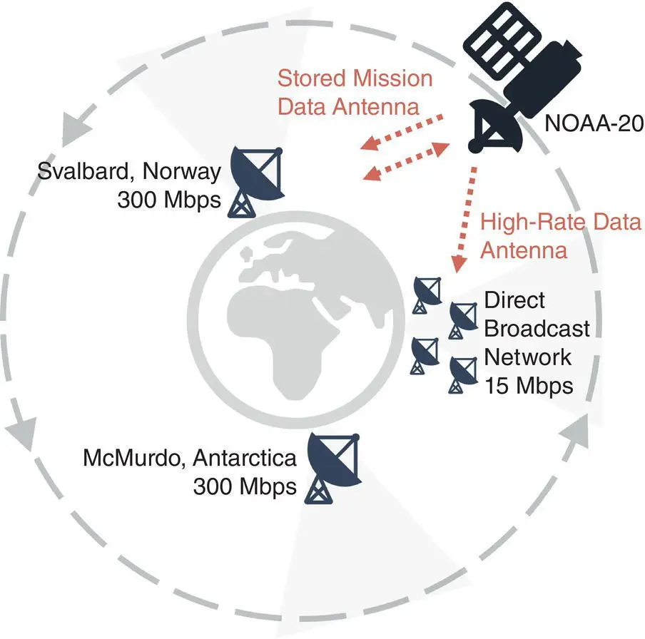
Figure 1.4 NOAA‐20 satellite downlink.

I have structured this book so that you can learn Python through a series of examples featuring real phenomena and public datasets. Some of the datasets and visualizations are useful for studying wildfires and smoke, dust plumes, and hurricanes. I will not cover all scenarios encountered in Earth science, but the skills you learn should be transferrable to your field. Some of these case studies include:

California Camp Fire (2018). California Camp Fire was a forest fire that began on November 8, 2018, and burned for 17 days over a 621 km2 area. It was primarily caused by very low regional humidity due to strong gusting wind events and a very dry surface. The smoke from the fire also affected regional air quality. In this case study, I will examine satellite observations to show the location and intensity as well as the impact that the smoke had on regional CO, ozone, and aerosol optical depth (AOD). Combined satellite channels also provide useful imagery for tracking smoke, such as the dust RGB product. Land datasets such as the Normalized Difference Vegetation Index (NDVI) are useful for highlighting burn scars from before and after the fire events.

Hurricane Michael (2018). Michael was a major hurricane that affect the Florida Panhandle of the United States. Michael developed as a tropical wave on October 7 in the southwest Caribbean Sea and grew into a Category 5 storm by October 10. Throughout its life cycle, Michael caused extensive flooding, leading to 74 deaths and $25 billion in damage. Several examples in this text utilize visible and infrared imagery of Hurricane Michael.

Louisiana Flood Event (2016). Thousands of homes were flooded in Louisiana when over 20 inches of rain fell between August 12 and August 21, 2016. The event began after a mesoscale convective system stalled over the area near Baton Rouge and Lafayette, Louisiana. I will use the IMERG global rainfall dataset to examine this event.

I have provided a brief overview of the many satellite missions and datasets that are available. This book has two main objectives: (1) to make satellite data and analysis accessible to the Earth science community through practical Python examples using real‐world datasets; and (2) to promote a reproducible and transparent scientific code philosophy. In the following chapters, I will focus on describing data conventions, common methods, and problem‐solving skills required to work with satellite datasets.

1 Tobin, D., Revercomb, H., Knuteson, R., Taylor, J., Best, F., Borg, L., et al. (2013). Suomi‐NPP CrIS radiometric calibration uncertainty. Journal of Geophysical Research: Atmospheres, 118(18), 10,589–10,600. https://doi.org/10.1002/jgrd.50809

2 Garner, R. (2015, July 10). ICESat‐2 Technical Requirements. www.nasa.gov/content/goddard/icesat‐2‐technical‐requirements

3 IBM (1989, January). Personal Computer Family Service Information Manual. IBM document SA38‐0037‐00. http://bitsavers.trailing‐edge.com/pdf/ibm/pc/SA38‐0037‐00_Personal_Computer_Family_Service:Information_Manual_Jul89.pdf