Magma Redox Geochemistry

Similarly, the redox potential related to Reaction 1.7is then:

(1.19)

Equations 1.18and 1.19, which can also be derived for Reactions 1.16and 1.17, can be used to trace E‐pH diagrams (also called Pourbaix or predominance diagrams; Casey, 2017) limiting the stability field of water ( Figure 1.1) and of any other systems in which E‐pH relationships can be established from the reactions of intervening species ( Figure 1.2). E‐pH diagrams are most used for understanding the geochemical formation, corrosion and passivation, leaching and metal recovery, water treatment precipitation, and adsorption.

For the set of species of interest, E‐pH diagrams show boundaries that are given by:

1 lines of negative slope that limit the stability field of water ( Equations 1.18and 1.19) or related to solid–solid phase changes in which paired electron–proton exchanges occur because the ligand (water) participates in reaction, such as in the case of the hematite–magnetite boundary in Figure 1.2: Figure 1.1 E‐pH diagram reporting the stability of water at T = 25°C and P = 1 bar for different partial pressure of H2 and O2 (log‐values).(1.20) Note that boundary slope is negative because protons and electrons appear on the same side of reaction. The protons/electrons ratio determines the slope value.

2 (rare) pH‐dependent lines of positive slopes, and associated with electron–proton exchanges involving, for example, reduction of dissolved cations to the oxide with a lower oxidation number, e.g.(1.21) Boundary slope is positive because protons and electons appear on different sides of reaction.

3 horizontal lines (pure electron exchange), such as in case of half‐reaction (1.22)which participates with half‐reaction 1.7in giving Reaction 1.3and does not involve explicitly the water solvent.

4 vertical lines, representing no change of oxidation state but only acid–base reactions (a sole exchange of protons for aqueous solutions), such as(1.23) with the boundary plotted at the pH value for which Q23 = K23 with aFe2O3(s) = (aFe3+)2 = 1 (and also aH2O = 1).

We now see that Reactions 1.3and 1.4are both related to half‐reaction 1.22, but they refer to different redox conditions and then have different meanings. In Reaction 1.3water is the oxidizing agent in acidic conditions, whereas it is the reducing agent in Reaction 1.4(Appelo and Postma, 1996), which represents a regulating mechanism of O 2, probably the oxidative alteration of rocks containing Fe 2+, in particular at oceanic ridges.

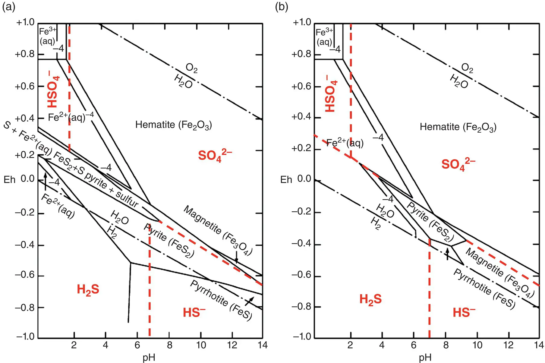
Figure 1.2 The E‐pH (Pourbaix) diagram for the Fe‐S‐H 2O system at 25°C at 1 bar total pressure and for total dissolved sulfur activities of 0.1 (panel a) and 10 –6(panel b). Superimposed are the stability fields for H 2S, HS –, HSO 4 2–and SO 4 2–dissolved species (red lines, traced from data in Biernat and Robins, 1969). Note how the field of stability of pyrite, FeS 2, shrinks and that of magnetite, Fe 3O 4, expands with decreasing total sulfur activity.

Modifed from Vaughan (2005).

Basically, E‐pH diagrams demonstrate that breaking of a redox reaction into half‐reactions is one of the most powerful ideas in redox chemistry, which allows relating the electron transfer to the charge transfer associated with the speciation state and the acid–base behavior of the solvent. Superimposing E‐pH diagrams allows a fast recognition of the existing chemical mechanism occurring in an electrolyte medium. For example, Figure 1.2on the Fe‐H‐O‐S system can be seen as the result of the superposition of stability diagrams for H‐O‐S and Fe‐O‐H system. The resulting diagram in Figure 1.2shows that the pyrite–magnetite boundary has a negative slope due to half‐reaction:

(1.24)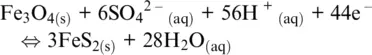

but also a positive slope well visible in Figure 1.2b due to sulfur reduction and dissolution in water as HS –:

(1.25)

Reaction 1.25implies of course a positive slope, because H +appears on the right side and electrons on the left. We can also appreciate the reduction of sulfur from pyrite to pyrrhotite at pH > 7:

(1.26)

which has a negative slope of –0.0295pH because the number of exchanged electrons is double than protons.

These concepts can then be transferred to other solvents in which ligand–metal exchanges lead to a different speciation state and are governed by a different notion of basicity, i.e. oxobasicity, such that (see Moretti, 2020 and references therein):

(1.27)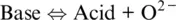

which can be also related to redox exchanges via the normal oxygen electrode ( Equation 1.6), in the same way the normal hydrogen electrode (Reaction 1.7) can be put in relation with the Bronsted‐Lowry definition of acid–base behaviour in aqueous solutions (see Moretti, 2020):

(1.28)

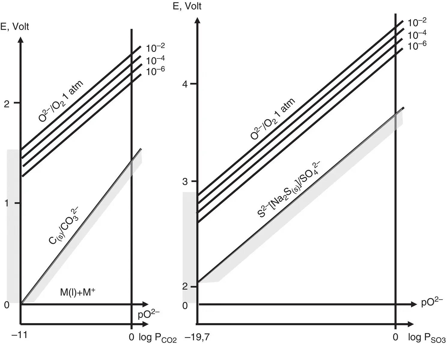
Figure 1.3 Limit of equilibrium potential‐pO 2–graphs in molten alkali carbonates and sulfates, at 600°C

(modified from Trémillon, 1974).

It is then possible to define pO 2–= ‐log a O 2–and introduce E‐pO 2–diagrams, in which acid species will be located at high pO 2–values. These diagrams were first introduced by Littlewood (1962) to present the electrochemical behaviour of molten salt systems and provide an understanding of the stability fields of the different forms taken by metals in these systems. Reference potential for molten salt is chosen either from anion or from cation, but anion, making up the ligand, is normally selected because there may be several different cations in the system.

For molten solvent diagrams, such as carbonate and sulfate melts, the stability area of the bath depends on the salt itself and can be seen by using as examples oxyanion solvents ( Figure 1.3). Limitations on the pO 2–scale of oxoacidity (Reaction 1.27) are given by the values of the Gibbs free energy of the formation reactions of alkali carbonates or sulfates at the liquid state, which depends on temperature as well as on pressure. On the basic side (low pO 2–side) the limit is imposed by the solubility threshold of the generic M ν+O ν/2oxide in the electrolyte medium, i.e., pO 2–min ≈ M ν+O ν/2solubility, whereas on the acidic side the limit is imposed by P CO2or P SO3= 1 bar. For example, it is 11 units in the case of the ternary eutectic Li 2CO 3+Na 2CO 3+K 2CO 3at 600°C and 19.7 units in the case of the ternary eutectic Li 2SO 4+ Na 2SO 4+ K 2SO 4at the same temperature (Trémillon 1974; Figure 1.3).