Machine Learning Techniques and Analytics for Cloud Security

In mathematics, linear models are well defined. For the purpose of predictive analysis, this model is commonly used nowadays. It uses a straight line to primarily address the relationship between a predictor and a dependent variable used as target. Basically, there exists two categories of linear regression, one is known as simple linear regression and the other one is known as multiple regressions. In linear regression, there could be independent variables which are either of type discrete or continuous, but it will have the dependent variables of type continuous in nature. If we assume that we have two variables, X as an independent variable and Y as a dependent variable, then a perfectly suited straight line is fit in linear regression model which is determined by applying a mean square method for finding the association between the independent variable X and the dependent variable Y. The relationship between them is always found to be linear. The key point is that in linear regression, the number of independent variable is one, but in case of multiple regressions, it can be one or more.

Although LR is commonly utilized for classification but it can effectively be applied in the field of regression also. The respondent variable being binary in nature can appear to any of the classes. The dependent variables aid in the process of predicting categorical variables. When there exists two classes and it is required to check where a new data point should belong, then a computing algorithm can determine the probability which ranges 0 to 1. LR model calculates the score of weighted summation of input and is given to the sigmoid function which activates a curve. The generated curve is popularly known as sigmoid curve ( Figure 3.1). The sigmoid function also known as logistic function generates a curve appears as a shapes like “S” and acquires any value which gets converted in the span of 0 and 1. The traditional method followed here is that when the output generated by sigmoid function is greater than 0.5, then it classifies it as 1, and if the resultant value is lower than 0.5, then it classifies it to 0. In case the generated graph proceeds toward negative direction, then predicted value of y will be considered as 0 and vice versa.

Building predictions by applying LR is quiet a simple task and is similar to numbers that are being plugged into the equation of LR for calculating the result. During the operating phase, both LR and linear regression proceeds in the same way for making assumptions of relationship and distribution lying within the dataset. Ultimately, when any ML projects are developed using prediction-based model then accuracy of prediction is always given preference over the result interpretation. Hence, any model if works good enough and be persistent in nature, then breaking few assumptions can be considered as relevant. As we have to work with gene expression, data belong to both normal and cancerous state and at the end want to identify the candidate genes whose expression level changes beyond a threshold level. This group of collected genes will be determined as genes correlated to cancer. So, the rest of the genes will automatically be excluded from the list of candidate genes. So, the whole task becomes a binary classification where LR fit well and has been used in the present work.

While learning the pattern with given data, then data with larger dimension makes the process complex. In ML, there are two main reasons why a greater number of features do not always work in favor. Firstly, we may fall victim to the “curse of dimensionality” that results in exponentially decreasing sample density, i.e., sparser feature space. Secondly, the more features we have, the more storage space and computation time we require. So, it can be concluded that excess amount of information is bad because the factors like quality and computational time complexity make the model inappropriate to fit. If the data is having huge dimension, then we should find a process for reduction of the same. But the process should be accomplished in such a manner where we can maintain the information which is significant as found in the original data. In this article, we are proposing an algorithm which serves that particular task. This is a very prominent algorithm and has been used extensively in different domain of work. It is named as Principal Component Analysis (PCA). PCA is primarily used to detect the highest variance dimensions of data and reshape it to lower dimensions. This is done in such a manner that the required information will be present, and when used by ML algorithms, it will have little impact on the perfection.

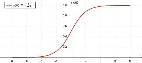
Figure 3.1 Sigmoid curve.

PCA transforms the data of higher dimension to lower dimension by incorporating a new coordinate system. In that newly introduced system, one axis is tagged as principal component which can express the largest amount of variance the data is having. In other way, it can simply be stated that the method PCA extracts the most significant variables from a large set of variables found in any available dataset and is marked as principal components. It retains most of the critical information from the actual dataset having higher dimension. The space defined in the new dimension designates the actual data in the form of principal component. It is important to understand how PCA is used to speed up the running time of the algorithm, without sacrificing much of the model performance and sometimes even improving it. As the most challenging part is which features are to be considered, the common tendency is to feed all the features in the model going to be developed. But doing so, the problem of over fitting in developed model will be introduced which is unlikely. So, to eliminate this problem two major things are considered, i.e., feature elimination and feature extraction. Feature elimination, i.e., somewhat arbitrarily dropping features, is problematic, given that, we will not obtain any information from the eliminated variables at all. Feature extraction, however, seems to circumvent this problem by creating new independent variables from the combination of existing variables. PCA is one such algorithm for feature extraction. In the process, it also drops the least important variables (i.e., performs feature elimination) but retains the combinations of the most important variables.

The aim of the proposed methodology presented in this article is to select a set of genes whose mutations have been observed in certain cancers. For accurate analysis and proper identification, the dataset belong to both carcinogenic and normal state has been examined. The main focus is to pick out some genes whose variations is observed in experiment and can be considered the most significant. These genes might be termed as the genes having association with cancer as because their expression level has been observed as crucially changed from their initial state. Finding these genes can have contribution in different ways to biologists, medical practitioners, pathologists, and many more. As we know that all genes do not mutate in all cancers, so our target is to segregate the genes which are mutated notably from their original state. The method first used PCA to reduce number of features (genes) which overcomes the curse of dimensionality and then LR is used for binary classification and identifies the set of genes which are expressed differentially [22, 23].

The implementation of our work started with gene expression data which is mathematically viewed as a set G = {g1, g2, g3,…, ga}. Each member giof Gcan be further expressed as gi = {gi1, gi2, gi3, …, gib}. Thus, the entire mathematical expression G can be considered as vector of vectors. In this context, g ican be thought as a vector/gene comprising of feature. More specifically, the entire dataset is represented in a matrix format of dimension a × b where a is number of genes and b is number of samples and a >> b. So, the number of samples is very less in compare to number of genes, considered as features. Two separate sets of data belong to two different states: normal and carcinogenic are taken here for generating the result from the proposed method. The whole dataset is represented mathematically as a set G = {G N, G C} where the dataset G Nrepresents normal or non-cancerous state and G Cbelongs to cancerous state. Two such datasets, viz ., lung and colon pertaining to non-cancerous and cancerous states, are studied to get experimental result, i.e., the set of genes whose mutations have been observed.