Machine Learning Techniques and Analytics for Cloud Security

In the present work, PCA is applied for the purpose of subgrouping the variables that preserves as much information present in the complete data as possible and also to speed up ML algorithm. The gene expression data G is presented here as a mathematical notation depicted as G ={g 1, g 2, g 3,…, g a}. The dataset used here belongs to two states, i.e., normal and cancerous states and treated here for determining the genes associated with cancer. The proposed algorithm works by reducing the size of features using PCA and then applying LR model on both datasets.

Here, we have applied LR as because the dependent variable (target) is categorical in nature. A threshold value has been considered here which helps to predict the class belongingness of a data. On the basis of the set threshold value, the predicted probability is realized for classification. After calculating the predicted value if found ≥ threshold limit, then gene is said to be cancerous in nature, otherwise non-cancerous. Considering x as independent variable and y as dependent variable in our LR model, the hypothesis function h ⊖(x) ranges between 0 and 1. As it works as a binary classifier, the result of prediction with the classification becomes y = 0 or y = 1. The hypothesis function h ⊖(x) actually can have values <0 or > 1. The mathematical expression in logistic classification used in the method is defined as 0 ≤ h ⊖(x) ≤ 1.

As in our Logistic Regression model, we want 0 ≤ h ⊖(x) ≤ 1, so our hypothesis function might be expressed as

(3.1)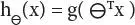

Replacing ⊖ Tx by t, the equation becomes

(3.2)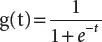

The above equation is known as sigmoid function

(3.3)

If “t” proceeds toward infinity, then the predicted variable Y will become 1. On the other hand, if “t” moves to infinity toward negative direction, then prediction of Y will be 0.

Mathematically this can be written as

(3.4)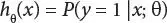

Computing the probability that y = 1 when x is given and it is parameterized by θ

(3.5)

(3.6)

While implementing the proposed method, we are selecting a bunch of r genes at random. This dataset of r × n (r denotes number of genes and n denotes number of samples) is partitioned into two sets, i.e., train and test. A certain percentage, say, p%, of the data is chosen as training set and rest is used as test set.

Features need to be scaled down before applying PCA. Standard scalar is used here for standardizing the features of the available dataset. Here, it is taken a onto unit scale (mean value is taken as 0 and variance is taken as 1). Now, PCA is applied with α as the number of parameters signified as components. It means that scikit-learn choose the minimum number of principal such that α% of the variance is retained.

After applying PCA, selected genes are fitted into the LR model. Test data and predicted data values are compared, and accuracy score is calculated. To obtain the gene with good accuracy score, the iterative LR and PCA was fitted at each iteration step and every time r random genes were selected. After the completion of the iterative process, the final list was sorted in descending order of the calculated accuracy score and top genes were selected.

From then “a” number of genes aC rdifferent combinations can be made by selecting r genes at random. Our algorithm works on M such combinations.

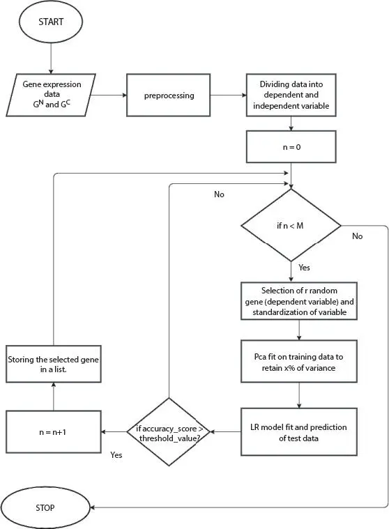
Figure 3.2 Flowchart of PC-LR algorithm.

Step 1: Read dataset G = {G N, G C} and make G = (G N) T∪(G C) T.

Step 2: Partition dataset into training and test dataset with a ratio.

Step 3: Standardize the dataset’s value onto unit scale.

Step 4: Repeat steps 5 to 9 till all genes are selected and processed.

Step 5: Selecting r genes at random and mark them.

Step 6: Applying PCA on selected genes to retain α% of the variance.

Step 7: Training the selected gene on Logistic Regression model.

Step 8: Predicting accuracy score by comparing the test data and predicted data

Step 9: If accuracy_score>threshold_value, then store these genes in a new list as resultant set of gene.

[end if]

Step 9: Stop

The pictorial representation of the algorithm gives clear idea of the working model ( Figure 3.2). The proposed algorithm works with gene expression dataset that belongs to both normal and cancerous state which is available in the form of a matrix where rows are genes and columns are the samples. The matrix is transposed so that samples were made as rows and all the genes were made as columns. So, this transposed matrix is given as the input. The whole dataset is partitioned into two categories: one is used for training purpose and the other one is for testing purpose. The model gets trained with the help of training data, and then, test data is used to measure the correctness of the model. The division of the data is done with the ratio 0.2 that means for training, 80% of the data is applied for training the model where as 20% data is applied for testing the same model.

The gene expression data values in the dataset vary in size. The numerical columns of the dataset need to be reduced to a common scale without any distortion of the differences lying in the range of values; therefore, standardization is needed to be used. Standardization is a form of scaling where the values are considered as centered on the basis of mean with a standard deviation taken as another component. Now, to start the iterative process for working a set of “r” genes were selected at random, and these genes were passed to train the model. Once these genes are selected, these are marked so that they will not be selected again in the iterative process. As in the dataset, it is observed that number of features (genes) is very large in compare to number of samples. In order to reduce curse of dimensionality, PCA was applied on the above selected “r” genes and a certain percentage, say, α%, of the variance is tried to be retained. Applying PCA, these genes were passed to train LR model. After training the model, test data is used to predict the outcome. Now, these predicted outcomes were checked against the actual outcomes of the test data and accuracy is calculated. If its accuracy level founds to be more than 85%, then these genes are extracted and stored in a list of candidate genes. The entire process gets repeated until all the genes were marked as selected in the dataset and accuracy was found to be considerate.