Reservoir Characterization

In the case of multiple bootstrap sampled training and test sets, ROC curve analysis has to deal with multiple ROC curves. In that case, quantiles of the true and false discovery rates, and quanties of area under ROC curve may be used for a compact description of a set of multiple ROC curves.

The writers distinguish two types of ROC curve analysis: (a) posterior ROC curve analysis, which is identical to traditional ROC curve analysis and (b) expected - posterior ROC curve analysis. Posterior ROC curve is a plot of posterior true discovery rate versus posterior false discovery rate, both calculated on the test set. Expected-posterior ROC curve is a plot of posterior true discovery rate (posterior TDR) versus expected false discovery rate (expected FDR), where posterior TDR is calculated on the test data and expected FDR assigned using training set data.

Figure 3.3shows histograms of posterior AUC values for three classifiers - divergence, sparsity, and distance. Sets of values of AD classifiers were created with bootstrap random sampling of the training and test sets. Each training set contained five records. The total number of randomly generated pairs of training and test sets was 1000. The intersections of continuous vertical black lines with x-axis at Figure 3.3shows the median value of the AUC. Dashed lines indicate lower and upper quantiles of the AUC distribution calculated for quantile probabilities Plow = 0.1 and Pupper = 0.9. According to the Figure 3.3, the divergence classifier is characterized by the narrowest distribution of AUC values and the largest AUC median. Distribution of this classifier is symmetric. Distributions of distance and sparsity classifiers are asymmetric with long tails in the direction of smaller values. As a result, lower quantiles for the distribution of distance and sparsity AUC are shifted towards smaller AUC values.

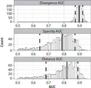
Figure 3.3 Histograms of area under posterior ROC Curve (AUC) for three anomaly detection classifiers. Size of each training set is 5 records.

Two of the three AD classifiers with AUC shown in Figure 3.3do not rely on the use of information about properties of petrophysical parameters within potential anomalies. This is their advantage since they may be used for detection of any type of anomaly with unknown properties. Although they underperform compared to the divergence classifiers that rely on the use of known anomaly properties, they still can produce median AUC values as high as 0.75.

Figure 3.4shows posterior AUC histograms for sparsity classifiers calculated for two sizes of the training sets. Continuous vertical lines are median values, intersection of doted lines with x-axis are the levels Plow =0.1 and Pupper =0.9. According to Figure 3.4, the AUC quantile region in the case of 25 records training sets is 40% narrower than the quantile region in the case of the training sets of 5 records.

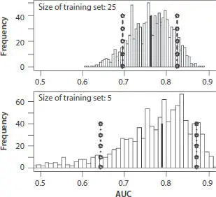
Figure 3.4 AUC histograms and quantile regions calculated from 1000 pairs of training-test sets. Size of the training sets: 5 and 25 records. Sparsity classifier.

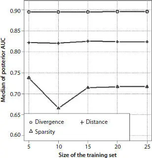
Figure 3.5 Median of posterior AUC for three AD classifiers as a function of the size of the training set.

The median of posterior AUC values and the width of the AUC quantile region for three AD classifiers are shown in Figures 3.5and 3.6. According to Figure 3.5, the median AUC of the divergence is higher than median AUC of other classifiers with its values stable around 0.9. Importantly, it is as high as 0.9 even for small training sets containing only five records. The sparcity classifier has the lowest AUC median which may be as small as 0.70.

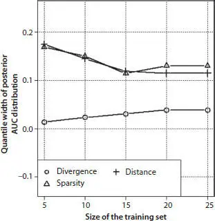
Figure 3.6 Quantile width of AUC distribution calculated on anomaly detection results from 1000 randomly generated pairs of training-test sets.

According to Figure 3.6, divergence has the narrowest AUC quantile region. AUC quantile regions of two other AD classifiers are significantly wider than that of divergence. The width of AUC quantile regions for these classifiers decreases with the increasing size of the training sets. It is still about three times as wide as the AUC quantile width of divergence for the size of training set 20, 25 records.

It was shown in the previous section that a divergence AD classifier is very efficient in detecting an anomaly with known properties. It was noted also that universal classifiers have lower efficiency compared to divergence.

The goal of this section is to develop a methodology for construction of an adaptive AD classifier working as a universal classifier for detection of anomalies of unknown type that is still almost as efficient as the specialized divergence classifier. The methodology for its synthesis is a two-step procedure:

1 1. Detection of a part of the anomaly using universal classifiers, such as the distance or the sparsity.

2 2. Optimization of aggregated classifier on the detected part of anomaly.

The structure of the aggregated classifier is defined by a set of coefficients sm (Eq. 3.7). These coefficients are chosen so that they maximize the ratio:

(3.8)

where sm ; 1 ≤ m ≤ M are weights and aggr() is defined by Eq. 3.7, classifier Anomaly Records are records identified by a universal classifier as anomaly, trainSetRecords are records from the training set.

To find coefficients sm that maximize efficiency criterion (3.8)we used a multidimensional grid search. In the grid search, the coefficients sm in Eq. 3.7take on a discrete set of values in the following region:

(3.9)

The efficiency criterion (3.8)is calculated for each combination of coefficients sm at individual grid nodes. An adaptive aggregated AD classifier maximizes efficiency criterion on the grid. As soon as the aggregated classifier is synthesized it may be used for anomaly detection using the test set.

We illustrate construction of an adaptive aggregated classifier using the sparsity classifier at the first optimization step. The classifier to be synthesized is of the following form:

(3.10)

Therefore, search is done on the two-dimensional grid.

Figure 3.7shows values of the sparsity classifier used as the first step of optimization of the aggregated classifier. Twenty regular records that form the training set are randomly selected out of a set of 50 records. The test set contains 30 regular and 25 anomaly records. Anomaly records are from gas-filled sands. Regular ones are from brine-filled sand or shale. The assigned value of the expected false discovery rate was 20%. Records classified as a potential anomaly include 13 actual anomaly records and 2 regular records. Thus the posterior true discovery rate is very moderate - 52%.