Electromagnetic Vortices
Здесь есть возможность читать онлайн «Electromagnetic Vortices» — ознакомительный отрывок электронной книги совершенно бесплатно, а после прочтения отрывка купить полную версию. В некоторых случаях можно слушать аудио, скачать через торрент в формате fb2 и присутствует краткое содержание. Жанр: unrecognised, на английском языке. Описание произведения, (предисловие) а так же отзывы посетителей доступны на портале библиотеки ЛибКат.
- Название:Electromagnetic Vortices
- Автор:
- Жанр:
- Год:неизвестен
- ISBN:нет данных
- Рейтинг книги:4 / 5. Голосов: 1
-
Избранное:Добавить в избранное
- Отзывы:
-
Ваша оценка:
Electromagnetic Vortices: краткое содержание, описание и аннотация
Предлагаем к чтению аннотацию, описание, краткое содержание или предисловие (зависит от того, что написал сам автор книги «Electromagnetic Vortices»). Если вы не нашли необходимую информацию о книге — напишите в комментариях, мы постараемся отыскать её.
, a team of distinguished researchers delivers a cutting-edge treatment of the research and development of electromagnetic vortex waves, including their related wave properties and several potentially transformative applications.
The book is divided into three parts. The editors first include resources that describe the generation, sorting, and manipulation of vortex waves, as well as descriptions of interesting wave behavior in the infrared and optical regimes with custom-designed nanostructures. They then discuss the generation, multiplexing, and propagation of vortex waves at the microwave and millimeter-wave frequencies. Finally, the selected contributions discuss several representative practical applications of vortex waves from a system perspective.
With coverage that incorporates demonstration examples from a wide range of related sub-areas, this essential edited volume also offers:
Thorough introductions to the generation of optical vortex beams and transformation optical vortex wave synthesizers Comprehensive explorations of millimeter-wave metasurfaces for high-capacity and broadband generation of vector vortex beams, as well as OAM detection and its observation in second harmonic generations Practical discussions of microwave SPP circuits and coding metasurfaces for vortex beam generation and orbital angular momentum-based structured radio beams and their applications In-depth examinations of OAM multiplexing using microwave circuits for near-field communications and wireless power transmission Perfect for students of wireless communications, antenna/RF design, optical communications, and nanophotonics,
is also an indispensable resource for researchers at large defense contractors and government labs.
Electromagnetic Vortices — читать онлайн ознакомительный отрывок
Ниже представлен текст книги, разбитый по страницам. Система сохранения места последней прочитанной страницы, позволяет с удобством читать онлайн бесплатно книгу «Electromagnetic Vortices», без необходимости каждый раз заново искать на чём Вы остановились. Поставьте закладку, и сможете в любой момент перейти на страницу, на которой закончили чтение.
Интервал:
Закладка:
Zhi Hao Jiang
Nanjing, P.R. China
Douglas H. Werner
University Park, PA, USA
1 Fundamentals of Orbital Angular Momentum Beams: Concepts, Antenna Analogies, and Applications
Anastasios Papathanasopoulos and Yahya Rahmat‐Samii
Department of Electrical and Computer Engineering, University of California, Los Angeles, CA, USA
1.1 Electromagnetic Fields Carry Orbital Angular Momentum
Angular momentum is the rotational equivalent of linear momentum. An object moving in a straight line carries linear momentum. Along with its linear motion, an object can also rotate in two distinct ways. A spinning object carries spin angular momentum (SAM) and an orbiting object carries orbital angular momentum (OAM), with Earth being an interesting example for consideration. The analogy between the angular momentum of a moving object and the electromagnetic wave’s angular momentum is shown in Figure 1.1. Earth’s spinning is associated with SAM; Earth’s orbital motion around the sun is linked to OAM. Electromagnetic beams may also carry these two types of momenta. If the electric field vector rotates along the beam axis, the beam has SAM; if the electromagnetic field’s wavefront is twisting, with the wave vector forming a helix, the beam has OAM.
The history of angular momentum dates back to the early twentieth century. The SAM of light was theoretically studied for the first time by Poynting in 1909 [1] and experimentally studied by Beth in 1936 [2]. SAM is intrinsic, since it does not depend on the choice of an axis, and it is only polarization dependent. If s is the SAM mode number, then s = ±1 corresponds to right‐ and left‐hand polarized waves, and s = 0 corresponds to linearly polarized waves. Although the experimental demonstration of the exchange of angular momentum between circularly polarized beams and matter was performed more than 80 years ago, the work associated with light’s angular momentum has been almost exclusively concerned with SAM.
It was not until 1992 that Allen et al. [3] showed that helically phased beams with a phase term e jlϕ(where  is the imaginary unit, l is the OAM mode number, and ϕ is the azimuthal angle) carry OAM. The wavefront of an OAM beam is a spiral; the phase twists around the beam axis and changes 2π l after a full turn. Unlike SAM, OAM is linked to spatial distribution rather than polarization. OAM is extrinsic, since it depends on the choice of the calculation axis. The angular momentum is the composition of SAM and OAM, such that the angular momentum mode number is j = s + l .
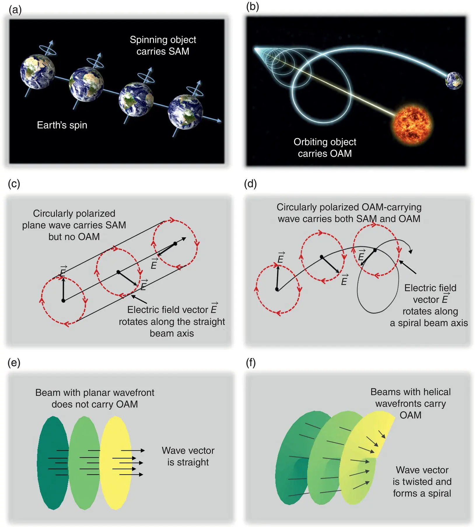
Figure 1.1 Analogy between moving object’s and electromagnetic wave’s angular momentum: (a) Earth spins and carries SAM; (b) Earth orbits around the sun and carries OAM; (c) a circularly polarized wave carries SAM; the electric field vector rotates along a straight beam axis; (d) a circularly polarized OAM‐carrying wave carries both SAM and OAM; the electric field vector rotates along a spiral beam axis; (e) beam with planar wavefront; the wavevector is straight; (f) OAM‐carrying beams with spiral wavefront; the wavevector is twisted.
1.2 OAM Beams; Properties and Analogies with Conventional Beams
Helically phased beams exhibit two unique properties: (i) the orthogonality of different OAM modes and (ii) the OAM beam divergence . As we will discuss in Section 1.3, the infinite number of orthogonal OAM modes provides an additional set of data carriers, thus OAM has the potential to increase the capacity and spectral efficiency of wireless communication links [4]. The beam divergence can be advantageous for applications that require cone‐shaped patterns, such as satellite‐based navigation and guidance systems that serve moving vehicles [5] but may also pose a challenge for long‐distance communication links [6]. In the subsequent paragraphs, these two peculiar features are explicated, and a comparative study between conventional and OAM beams is performed to underline their differences.
The first characteristic property of OAM beams is the orthogonality of distinct OAM modes. In general, the electric field of an OAM beam can be written as:
(1.1) 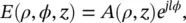
where ρ is the radial distance, ϕ is the azimuthal angle, and z is the propagation distance in the cylindrical coordinate system. There exist various subsets of OAM‐carrying beams, for example Laguerre–Gaussian [3], Bessel–Gaussian [7], hypergeometric–Gaussian [8], vector vortex [9], and other beams [10]. The radial distribution A ( ρ , z ) in Eq. (1.1)defines the special subset among all OAM‐carrying beams. All the previous beams carry the e jlϕterm, which gives rise to an OAM mode of l ‐order. If we consider the electric fields E 1( ρ , ϕ , z ), E 2( ρ , ϕ , z ) of two OAM beams with modes l 1, l 2, and radial distributions A 1( ρ , z ), A 2( ρ , z ), the following orthogonality relation is satisfied [11]:
(1.2) 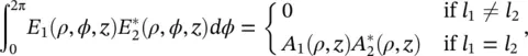
where the asterisk ( *) denotes the complex conjugate. It follows that: (i) there is an infinite number of OAM modes, with each mode identified by the mode number l , and (ii) the infinite set of OAM states forms an orthogonal basis.
The second special feature of OAM beams is the beam divergence . The far‐field signature of the helical wavefront is an amplitude null at the phase vortex center. Accordingly, the null size can be described in terms of a divergence angle, which represents the angle from the null to the maximum gain [12]. As the OAM beam travels through space, the radius of the ‘dark zone’ around the amplitude null in the center of the beam increases.
1.2.1 Laguerre–Gaussian Modes
In general, an OAM‐carrying beam could refer to any beam that carries the e jlϕterm, regardless of the radial distribution A ( ρ , z ) in Eq. (1.1). The Laguerre–Gaussian modes are a special subset among all OAM‐carrying beams that are cylindrically symmetric solutions to the paraxial wave equation in the cylindrical coordinate system [3]. The Laguerre–Gaussian modes are chosen to be presented because they are one of the most popular examples of OAM‐carrying beams (see, for example [13–18]), and a general OAM‐carrying beam can be expanded in a complete basis of Laguerre–Gaussian modes [11, 19, 20]. The electric field of a linearly polarized Laguerre-Gaussian beam at z = 0 can be written as [3, 5]:
(1.3) 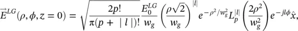
Интервал:
Закладка:
Похожие книги на «Electromagnetic Vortices»
Представляем Вашему вниманию похожие книги на «Electromagnetic Vortices» списком для выбора. Мы отобрали схожую по названию и смыслу литературу в надежде предоставить читателям больше вариантов отыскать новые, интересные, ещё непрочитанные произведения.


Обсуждение, отзывы о книге «Electromagnetic Vortices» и просто собственные мнения читателей. Оставьте ваши комментарии, напишите, что Вы думаете о произведении, его смысле или главных героях. Укажите что конкретно понравилось, а что нет, и почему Вы так считаете.