Distributed Acoustic Sensing in Geophysics

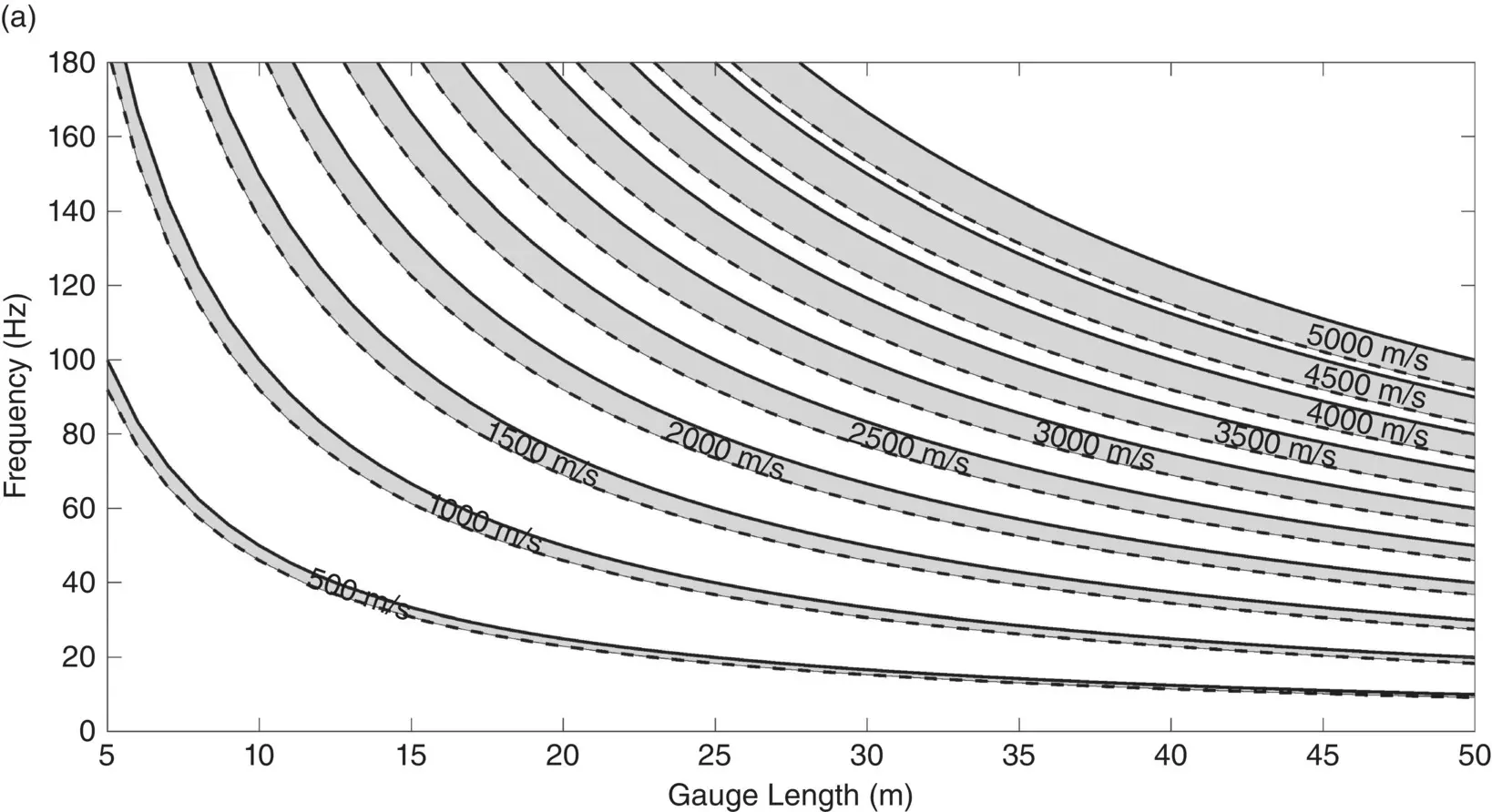
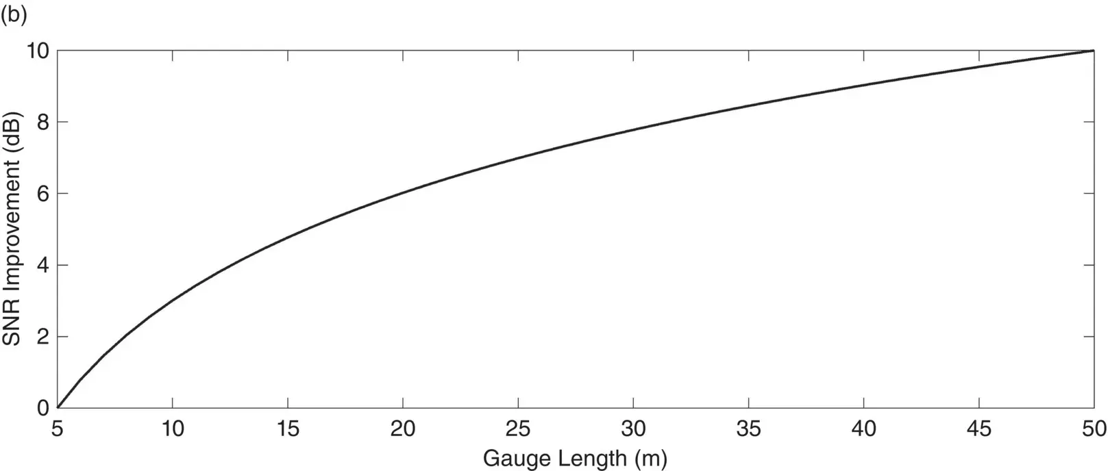
Figure 2.3 (Top) Location of first spectral notch for a range of gauge lengths; solid black line represents the spectral notch associated with the labeled velocity, and the dotted line represents the corresponding −20 dB point. (Bottom) Relative signal‐to‐noise improvement using different gauge lengths compared to a 5 m gauge.

Two trends are easily observed: (1) larger gauge lengths can be used if the apparent velocities of interest are large, and (2) spectral notches are not as limiting on the upper frequencies for small gauges. It might appear that the conclusion should be to always use a small gauge length; but, as previously mentioned, the SNR improves as the gauge length increases ( Figure 2.3, bottom). The vertical axis shows the SNR improvement as compared to a 5 m gauge, in dB; thus, the improvement using a 15 m gauge is 4.8 dB, while the 40 m gauge provides 9 dB improvement. Therefore, the goal is to use as large a gauge length as possible without damaging the desired frequency content of the seismic waves being recorded.

For earthquake‐monitoring applications where the frequency content is typically much less than 2 Hz, the notches will not affect the recorded spectrum, and thus a long gauge is appropriate. For a Gulf of Mexico deepwater VSP, it could be that seismic energy reflecting from the reservoir has a maximum frequency content of 20 Hz because of the earth’s attenuation. Figure 2.3(top) shows that any gauge length from 5 to 50 m can capture all seismic waves faster than 1000 m/s; thus, it might be worth the added SNR benefits to use a long gauge. However, if, instead, the application is shallow and unconsolidated formations with extremely slow P‐ and S‐waves, and a high‐frequency source is used, then an extremely short gauge should be used at the expense of SNR.

The IU sends a pulse of light into the fiber with a sampling rate of 10 kHz or higher. The time between these pulses are set so that the light has time to reach the end of the fiber and return as backscattered energy to the photodetector in the IU. The longer the sensing fiber, the slower this sampling rate should be, so that the pulse of light has the necessary time to return to the IU without interfering with another pulse.

Pulse width is another important parameter to choose. The pulse of light sent by the IU into the fiber should be limited in time duration so that it does not impede the functionality of the interferometer. Strain measurement is created from the interference of the pulse of light going through both the direct (short) path and the long path through the gauge length delay coil. The time duration of the pulse should be chosen so that backscattered energy from the short path does not interfere or overlap with the time window containing the backscatter energy traveling along the long path. Figure 2.4shows the suggested pulse widths associated with gauge lengths. The value of using a long pulse width as compared to a short one is that more light enters the fiber, and an improved SNR is obtained; however, if the pulse width used is too long so that the time footprint of the pulse is longer than the gauge length, the quality of the strain measurement drops.

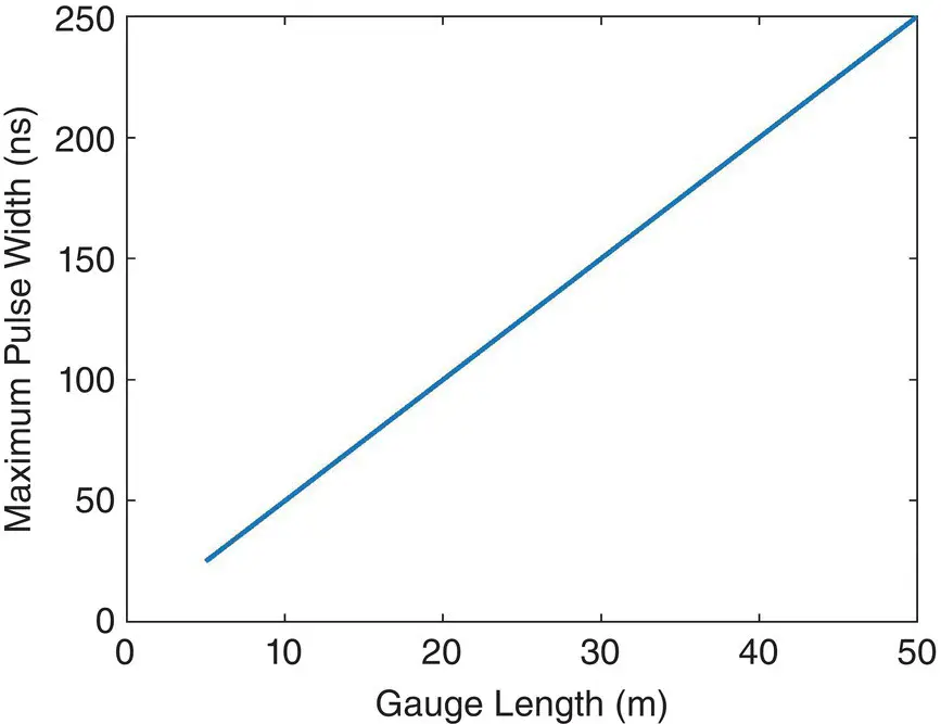
Figure 2.4 Recommended pulse width as a function of gauge length.

One unique property of all DAS data, compared to conventional seismic data, is the occurrence of channel fading, which is also called “vertical noise” because it appears as vertical stripes on a record where time is plotted on the vertical axis and channel number (or depth) on the horizontal axis. As discussed in the IU section, relative strain data are computed from the I and Q traces. The stability of extracting the phase term using Equation 2.1depends upon the signal fidelity of both the I and Q traces. Because of the interaction of the backscattered light created from the distribution of random scattering sites in the fiber, there are occasions when the intensity of the backscattered light is low, causing the length (modulus) of the I/Q vector to be comparatively small in numerical value ( Figure 2.2, right) and thus more subject to noise. This, in turn, makes taking the arctangent of Q/I to become extremely noisy. While the computation of the arctangent is stable, the phase‐unwrapping algorithm is unable to determine the appropriate value of π to add to the phase to create a continuous signal, creating unexpected jumps in phase at these times on the trace.

The occurrence of fading changes in both time and distance along the fiber; for example, extremely small changes in the fiber’s temperature move the scattering sites and cause temporary dimming of the backscattered signal at new locations. It has been observed (Ellmauthaler et al., 2016) that approximately 3% of the fiber is faded at any given moment; for example, if the sensing fiber has 5,000 channels, that translates to as many as 150 channels exhibiting some form of fading. However, even during small time intervals of approximately 1 min, the fading on the affected channels will move. Thus, if it is possible to repeat the source and take multiple measurements, it is easy to obtain reliable data eventually without fading.

Figure 2.5shows simulated fading on a single channel. The top panel shows the I trace (blue) and Q trace (orange). In addition to the desired seismic signal, a temperature drift was simulated by a long period trend. Notice that, between 2 and 2.25 sec, the amplitudes of both I and Q traces diminish toward zero. The middle panel shows the resulting relative strain trace computed from the I and Q traces. The relative strain trace is continuous and smooth before and after this time interval. However, during the dimmed interval, it is evident that the phase‐unwrapping algorithm has failed to unwrap the phase properly, and multiple non‐physical jumps in the strain trace occur. Notice that the temperature drift shows up as a background “ramp” on the relative strain data. The bottom panel shows the strain rate trace, which is simply the time derivative of the relative strain trace. Jumps in the relative strain trace become negative and positive spikes in the strain rate trace. The strain rate data is not as sensitive to the temperature drift since the time derivative is similar to a low‐cut filter and has greatly reduced the long period temperature ramp.

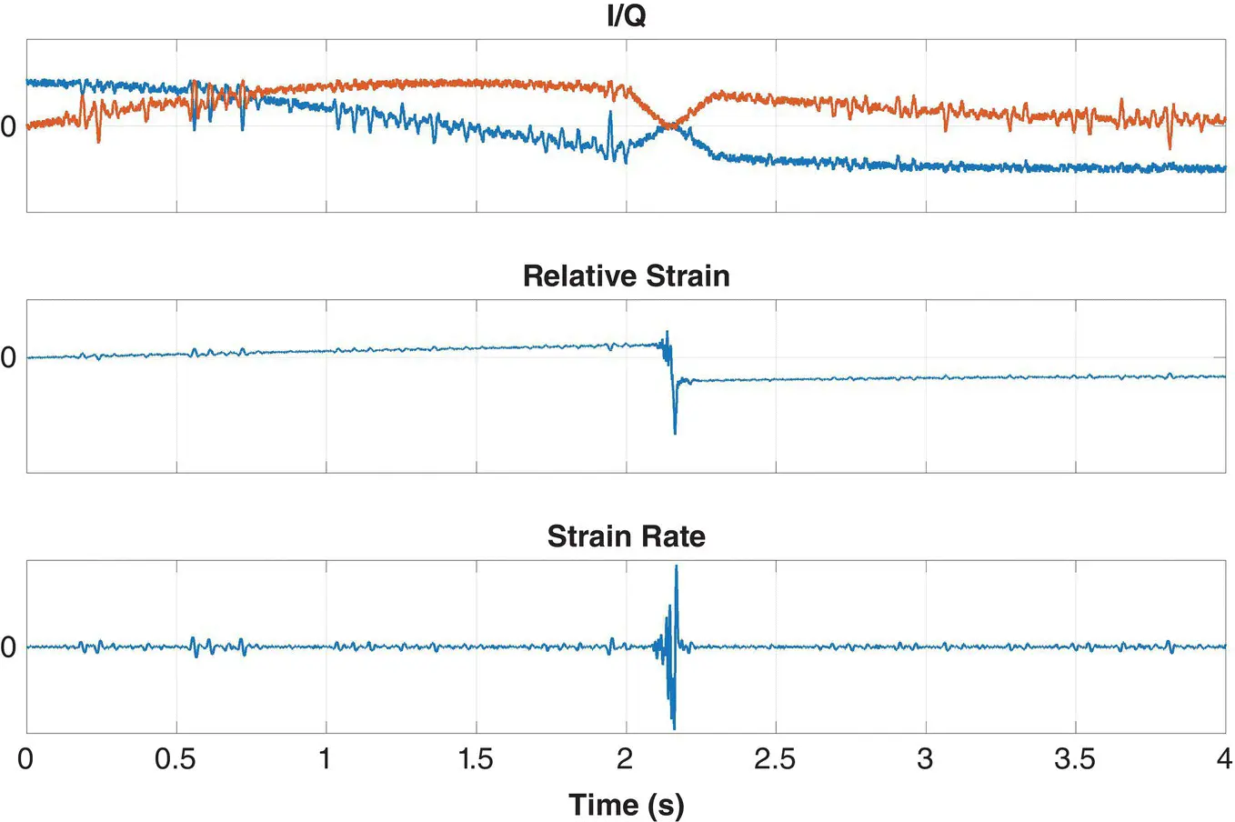
Figure 2.5 (Top) I (blue) and Q (orange) traces; (middle) corresponding relative strain; (bottom) strain rate.

It is difficult to perform conventional processing and analysis of the resulting seismic data without addressing these faded channels in either the relative strain or strain rate data. Figure 2.6shows an example of strain rate DAS VSP data collected using a vibrator source with a 12 sec sweep and 4 sec listen time. The top two panels for Figure 2.6show an uncorrelated trace without and with fading, respectively. Notice the spikes between 10 and 12 sec on the faded trace. The bottom two panels on Figure 2.6show the corresponding correlated traces; it is evident that the spikes in the faded trace have affected the entire trace because of the correlation process. For land data, where it is possible to acquire multiple sweeps at the same shot point, the spikes caused by fading can be mitigated using a weighted stacking of the sweeps, which minimizes large amplitude spikes. For marine data, where typically only one “pop” is acquired at each shot point, a despiking algorithm can be used to remove the faded portions of the trace before further processing and analysis.