Stephen Winters-Hilt - Informatics and Machine Learning

As N ➔∞ get the LLN (weak):

If X kare iid copies of X , for k = 1,2,…, and X is a real and finite alphabet, and μ = E ( X ), σ 2= Var( X ), then: P (| N− μ | > k )➔0, for any k > 0. Thus, the arithmetic mean of a sequence of iid r.v.s converges to their common expectation. The weak form has convergence “in probability,” while the strong form has convergence “with probability one.”

Here, we talk of the probability of seeing something after k tries when the probability of seeing that event at each try is “ p .” Suppose we see an event for the first time after k tries, that means the first ( k − 1) tries were nonevents (with probability (1 − p ) for each try), and the final observation then occurs with probability p , giving rise to the classic formula for the geometric distribution:

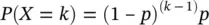
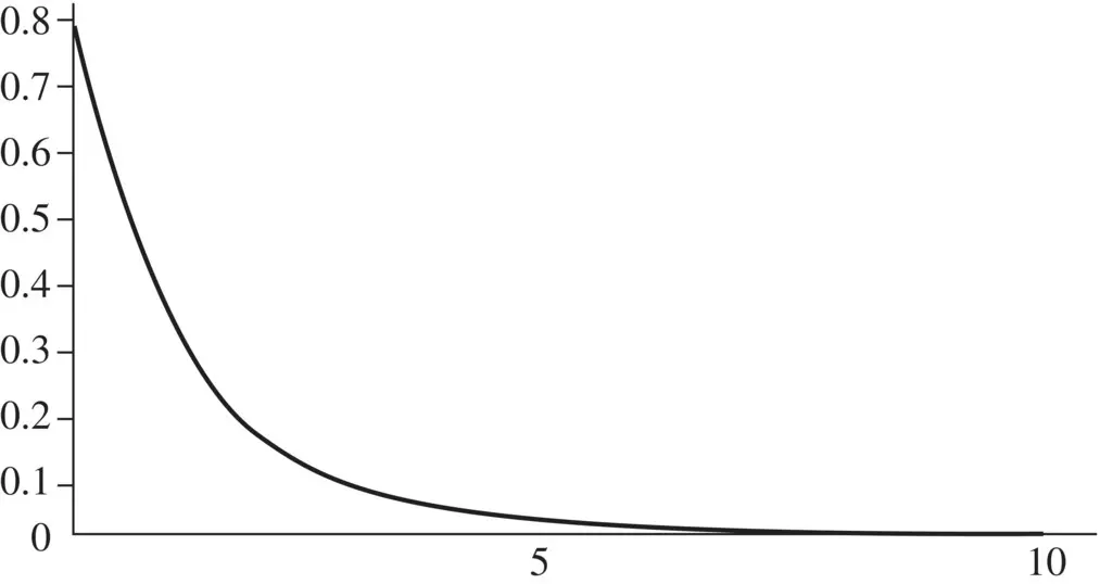
Figure 2.3 The Geometric distribution, P ( X = k ) = (1 − p ) (k−1) p , with p = 0.8.

As far as normalization, i.e. do all outcomes sum to one, we have:

Total Probability = ∑ k = 1(1 – p ) (k−1) p = p [1 + (1 – p ) + (1 – p ) 2+ (1 – p ) 3+ …] = p [1/(1 − (1 − p ))] = 1

So total probability already sums to one with no further normalization needed. In Figure 2.3is a geometric distribution for the case where p = 0.8:

For the Normal distribution the normalization is easiest to get via complex integration (so we'll skip that). With mean zero and variance equal one ( Figure 2.4) we get:

Nongeometric duration distributions occur in many familiar areas, such as the length of spoken words in phone conversation, as well as other areas in voice recognition. Although the Gaussian distribution occurs in many scientific fields (an observed embodiment of the LLN, among other things), there are a huge number of significant (observed) skewed distributions, such as heavy‐tailed (or long‐tailed) distributions, multimodal distributions, etc.

Heavy‐tailed distributions are widespread in describing phenomena across the sciences. The log‐normal and Pareto distributions are heavy‐tailed distributions that are almost as common as the normal and geometric distributions in descriptions of physical phenomena or man‐made phenomena. Pareto distribution was originally used to describe the allocation of wealth of the society, known as the famous 80–20 rule, namely, about 80% of the wealth was owned by a small amount of people, while “the tail,” the large part of people only have the rest 20% wealth. Pareto distribution has been extended to many other areas. For example, internet file‐size traffic is a long‐tailed distribution, that is, there are a few large sized files and many small sized files to be transferred. This distribution assumption is an important factor that must be considered to design a robust and reliable network and Pareto distribution could be a suitable choice to model such traffic. (Internet applications have many other heavy‐tailed distribution phenomena.) Pareto distributions can also be found in a lot of other fields, such as economics.

Figure 2.4 The Gaussian distribution, aka Normal, shown with mean zero and variance equal to one: N x( μ , σ 2) = N x(0,1).

Log‐normal distributions are used in geology and mining, medicine, environment, atmospheric science, and so on, where skewed distribution occurrences are very common. In Geology, the concentration of elements and their radioactivity in the Earth's crust are often shown to be log‐normal distributed. The infection latent period, the time from being infected to disease symptoms occurs, is often modeled as a log‐normal distribution. In the environment, the distribution of particles, chemicals, and organisms is often log‐normal distributed. Many atmospheric physical and chemical properties obey the log‐normal distribution. The density of bacteria population often follows the log‐normal distribution law. In linguistics, the number of letters per words and the number of words per sentence fit the log‐normal distribution. The length distribution for introns, in particular, has very strong support in an extended heavy‐tail region, likewise for the length distribution on exons or open reading frames (ORFs) in genomic deoxyribonucleic acid (DNA). The anomalously long‐tailed aspect of the ORF‐length distribution is the key distinguishing feature of this distribution, and has been the key attribute used by biologists using ORF finders to identify likely protein‐coding regions in genomic DNA since the early days of (manual) gene structure identification.

A series is a mathematical object consisting of a series of numbers, variables, or observation values. When observations describe equilibrium or “steady state,” emergent phenomenon familiar from physical reality, we often see series phenomena that are martingale. The martingale sequence property can be seen in systems reaching equilibrium in both the physical setting and algorithmic learning setting.

A discrete‐time martingale is a stochastic process where a sequence of r.v. { X 1, …, X n} has conditional expected value of the next observation equal to the last observation: E ( X n+1| X 1, … X n) = X n, where E (| X n|) < ∞. Similarly, one sequence, say { Y 1,…, Y n}, is said to be martingale with respect to another, say { X 1,…, X n}, if for all n : E ( Y n+1| X 1, … X n) = Y n, where E (| Y n|) < ∞. Examples of martingales are rife in gambling. For our purposes, the most critical example is the likelihood‐ratio testing in statistics, with test‐statistic, the “likelihood ratio” given as: Y n= Π n i=1 g( X i)/ f( X i), where the population densities considered for the data are fand g. If the better (actual) distribution is f, then Y nis martingale with respect to X n. This scenario arises throughout the hidden Markov models (HMM) Viterbi derivation if local “sensors” are used, such as with profile‐HMM's or position‐dependent Markov models in the vicinity of transition between states. This scenario also arises in the HMM Viterbi recognition of regions (versus transition out of those regions), where length‐martingale side information will be explicitly shown in Chapter 7, providing a pathway for incorporation of any martingale‐series side information (this fits naturally with the clique‐HMM generalizations described in Chapter 7). Given that the core ratio of cumulant probabilities that is employed is itself a martingale, this then provides a means for incorporation of side‐information in general (further details in Appendix C).