Stephen Winters-Hilt - Informatics and Machine Learning
Здесь есть возможность читать онлайн «Stephen Winters-Hilt - Informatics and Machine Learning» — ознакомительный отрывок электронной книги совершенно бесплатно, а после прочтения отрывка купить полную версию. В некоторых случаях можно слушать аудио, скачать через торрент в формате fb2 и присутствует краткое содержание. Жанр: unrecognised, на английском языке. Описание произведения, (предисловие) а так же отзывы посетителей доступны на портале библиотеки ЛибКат.
- Название:Informatics and Machine Learning
- Автор:
- Жанр:
- Год:неизвестен
- ISBN:нет данных
- Рейтинг книги:3 / 5. Голосов: 1
-
Избранное:Добавить в избранное
- Отзывы:
-
Ваша оценка:
Informatics and Machine Learning: краткое содержание, описание и аннотация
Предлагаем к чтению аннотацию, описание, краткое содержание или предисловие (зависит от того, что написал сам автор книги «Informatics and Machine Learning»). Если вы не нашли необходимую информацию о книге — напишите в комментариях, мы постараемся отыскать её.
Discover a thorough exploration of how to use computational, algorithmic, statistical, and informatics methods to analyze digital data Informatics and Machine Learning: From Martingales to Metaheuristics
ad hoc, ab initio
Informatics and Machine Learning: From Martingales to Metaheuristics
Informatics and Machine Learning — читать онлайн ознакомительный отрывок
Ниже представлен текст книги, разбитый по страницам. Система сохранения места последней прочитанной страницы, позволяет с удобством читать онлайн бесплатно книгу «Informatics and Machine Learning», без необходимости каждый раз заново искать на чём Вы остановились. Поставьте закладку, и сможете в любой момент перейти на страницу, на которой закончили чтение.
Интервал:
Закладка:
For k > 0, P (| X − E ( X )| > k ) ≤ Var( X )/ k 2
Proof: 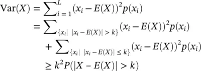
2.5 Statistics, Conditional Probability, and Bayes' Rule
So far we have counts and probabilities, but what of the probability of X when you know Y has occurred (where X is dependent on Y )? How to account for a greater state of knowledge? It turns out the answer to this was not put on a formal mathematical footing until half way thru the twentieth century, with the Cox derivation [101] .
2.5.1 The Calculus of Conditional Probabilities: The Cox Derivation
The rules of probability, including those describing conditional probabilities, can be obtained using an elegant derivation by Cox [101] . The Cox derivation uses the rules of logic (Boolean algebra) and two simple assumptions. The first assumption is in terms of “ b|a ,” where b|a ≡ “likelihood” of proposition b when proposition a is known to be true. (The interpretation of “likelihood” as “probability” will fall out of the derivation.) The first assumption is that likelihood c‐and‐b|a is determined by a function of the likelihoods b|a and c|b‐and‐a :
(Assumption 1) c ‐and‐ b | a = F ( c | b ‐and‐ a , b | a ),
for some function F . Consistency with the Boolean algebra then restricts F such that ( Assumption 1)reduces to:

where f is a function of one variable and C is a constant. For the trivial choice of function and constant there is:

which is the conventional rule for conditional probabilities (and c‐and‐b|a is rewritten as p ( c,b|a ), etc.). The second assumption relates the likelihoods of propositions b and ~ b when the proposition a is known to be true:
(Assumption 2)~ b | a = S ( b | a ),
for some function S . Consistency with the Boolean algebra of propositions then forces two relations on S :

which together can be solved to give:
where m is an arbitrary constant. For m = 1 we obtain the relation p ( b|a ) + p (~ b|a ) = 1, the ordinary rule for probabilities. In general, the conventions for Assumption 1can be matched to those on Assumption 2, such that the likelihood relations reduce to the conventional relations on probabilities. Note: conditional probability relationships can be grouped:

to obtain the classic Bayes Theorem.
2.5.2 Bayes' Rule
The derivation of Bayes’ rule is obtained from the property of conditional probability:

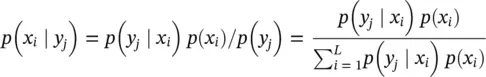
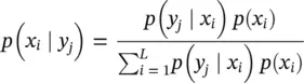
Bayes' Rule provides an update rule for probability distributions in response to observed information. Terminology:
p(xi ) is referred to as the “prior distribution on X” in this context.
p(xi ∣ yj ) is referred to as the “posterior distribution on X given Y.”
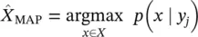
2.5.3 Estimation Based on Maximal Conditional Probabilities
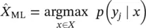
There are two ways to do an estimation given a conditional problem. The first is to seek a maximal probability based on the optimal choice of outcome (maximum a posteriori [MAP]), versus a maximal probability (referred to as a “likelihood” in this context) given choice of conditioning (maximum likelihood [ML]).
MAP Estimate:
Provides an estimate of r.v. X given that Y = y jin terms of the posterior probability:
ML Estimate:
Provides an estimate of r.v. X given that Y = y jin terms of the maximum likelihood:
2.6 Emergent Distributions and Series
In this section we consider a r.v., X , with specific examples where those outcomes are fully enumerated (such as 0 or 1 outcomes corresponding to a coin flip). We review a series of observations of the r.v., X , to arrive at the LLN. The emergent structure to describe a r.v. from a series of observations is often described in terms of probability distributions, the most famous being the Gaussian Distribution (a.k.a. the Normal, or Bell curve).
2.6.1 The Law of Large Numbers (LLN)
The LLN will now be derived in the classic “weak” form. The “strong” form is derived in the modern mathematical context of Martingales in Appendix C.1.
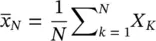
Let X kbe independent identically distributed (iid) copies of X , and let X be the real number “alphabet.” Let μ = E ( X ), σ 2= Var( X ), and denote

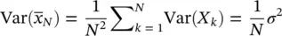
From Chebyshev: P ( |  N− μ |> k ) ≤ Var(
  N)/ k 2=
  σ 2
σ 2
Интервал:
Закладка:
Похожие книги на «Informatics and Machine Learning»
Представляем Вашему вниманию похожие книги на «Informatics and Machine Learning» списком для выбора. Мы отобрали схожую по названию и смыслу литературу в надежде предоставить читателям больше вариантов отыскать новые, интересные, ещё непрочитанные произведения.


Обсуждение, отзывы о книге «Informatics and Machine Learning» и просто собственные мнения читателей. Оставьте ваши комментарии, напишите, что Вы думаете о произведении, его смысле или главных героях. Укажите что конкретно понравилось, а что нет, и почему Вы так считаете.