Handbook of Intelligent Computing and Optimization for Sustainable Development

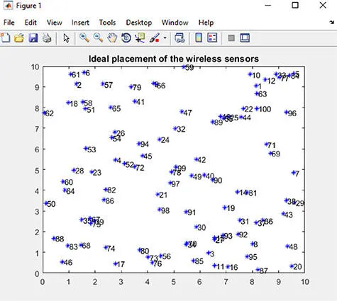
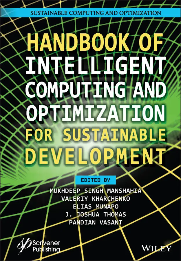
Figure 6.18 Ideal placement of nodes.

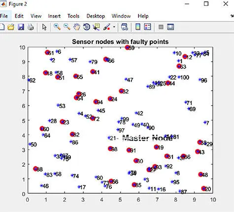
Figure 6.19 Sensor nodes with faulty points.

Now, we will separate out the faulty nodes from the whole nodes. To separate out faulty nodes formula is p = 40 where p is percentage of faulty nodes out of the total number of nodes.

Types of Faulty Nodes

We have four types of faulty nodes

1 1. Permanent

2 2. Transient

3 3. Intermittent

4 4. Dynamic

Now, assign the x and y coordinates of faulty nodes and initiate the master node and calculate the distance of each faulty nodes from master nodes by mean square root formula, also the time from the master node to the faulty nodes. Plot the all four types (permanent, transient, intermittent, and dynamic) faulty nodes in the figure.

By subtracting the faulty nodes from the equation, we will get the best match from up nodes, down nodes, left nodes and right nodes indexes. To get best match, we calculate the transfer information from sender to receiver node. All nodes toward the receiver, calculate the horizontal distance between “coor1” and “r_coor” and vertical distance between “coor1” and “r_coor”.

Now, there are three conditions or cases. First two cases in which sender and receiver are outbound and third case is wen sender and receiver is inbound. But for third case, there are four scenarios.

1 1. Scenario with no error.

2 2. Scenario with error.

3 3. Scenario with path hoping.

4 4. Scenario with errors and correction.

But, here we will discuss three cases of scenario without and with errors and with errors and correction.

a. Case without errorsIn scenario without errors, we will first transfer the information of sender and reliever nodes. Now, check the range and distance between the nodes. Next step is to generate the blinking line and check the set of nodes (faulty nodes) and then send the information to the destination with the help of coordinates of x and y. In this figure, sender 21 is sending packet to the receiver through the minimum path and time delay. It passes through 3 nodes (72, 54, 65).

b. Case with errorIn scenario with error, loop will run until the coordinate 1 is equal to the coordinate of receiver. After reaching at the receiver node, now find the coordinate 2 from the valid group of nodes (avoid faulty node). In this figure, 72 is faulty node and it stops the procedure but again scenario will generate another loop to reach at the receiver node. This time they avoid 72 and pass through 52, 54, and 57 or 45, 26, and 57. It is shorter path than the without errors.

c. Case with error detection and correctionThird scenario is with errors and correction. This is proposed scenario in which we will simulate the loop with errors and then correct the errors to find out the best way to reach at the destination node. To correct the errors, we will change the way/nodes that are faulty in the whole scenario and choose another node for the receiver node. The simulation of such scenario is shown in figure. It will pass through.

The delays calculation and simulation results for different scenario are presented in Figure 6.20.

Packet delivered out of 100 for first path: 60.9696 in which we face no errors during the simulation of VANETs. Packet delivered out of 100 for second path: 86.9899 in which we face errors during simulation and we started the loop from the start and delivered the packet. Packet delivered out of 100 for third path: 86.9899 in which we corrected the error and successfully delivered the packet from sender to receiver as shown in Figure 6.21.

Figure 6.20 Delay.

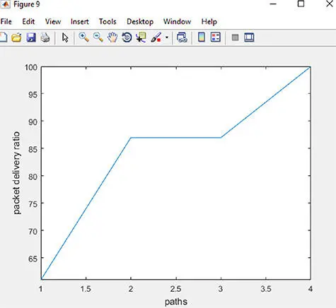
Figure 6.21 Packet delivery ratio.

Energy is the parameter in which energy absorbed by a node during the transformation of information from sender to receiver in scenario with errors more energy is used than scenario without error as shown in Figure 6.22.

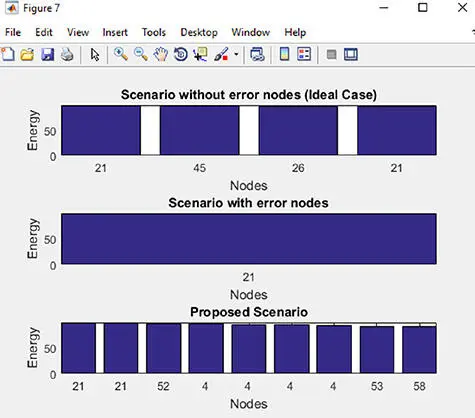
Figure 6.22 Throughput .

nodex_g, nodey_g, nodex, nodey_e, nodex, nodey, good_node, and enc are deploy nodes. High = 10 (upper bound for node value) low = 0(lower bound for node value). Next is to enter the number of nodes. We will calculate good and bad nodes from the total nodes, and at the end display the nodes consisting of three protocols as depicted in Figure 6.23.

Figure 6.23 Placement of nodes.

Now, enter the source and receiver node from the total displaced nodes. Put the values of sender and receiver node. Now, put range of node which is 2 here. Assign the sender coordinates and draw the circle by the function.

Find out the fault in routes and times in delivery. Next is the procedure of number of steps. First is to finding nodes which are in range to the sender nodes, calculate distances of senders with nodes in its range, indexes of ranged nodes with respect to sender, calculate distance between sender and all other nodes, select only the nodes in range. Now, make group of ranged nodes, and then, apply DE and find cost of all the groups collected. Selecting node combination with best cost, finding the closest node to the receiver, out of the selected ranged nodes, distance of the ranged nodes to receiver, arranging the indexes. Now, find the next node to hop on, from next hop to the receiver node draw the line and circle.

For fitness function, we have many trust measurement alpha = 0.6, beta = 0.4, DP_f = 1, CP_f = 1, T_ab = alpha*DP_f + beta*CP_f, residual battery life, E = 100 (Enter power for each node), Ef = 60 (Enter power required to forward single packet), Eq = 30 (Enter dissipated power of the equipment), RBL = E/(Ef + Eq), hop count, fitness function, k1 = 0.1, fit = (Hopcount*k1) + (1 − T_ab) + (1/RBL), as shown in Figure 6.24.

After the fitness function, simulation start generating results in green and red nodes while green are good and red are bad nodes as presented in Figure 6.25.

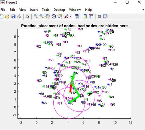
Figure 6.24 Good and bad nodes.