Nathalie Peyrard - Statistical Approaches for Hidden Variables in Ecology

A further question concerns the extent to which activity is influenced by covariates (distance from a point of interest, time of day, etc.). One way of including covariates is to model their impact on the transition between activities (Calenge et al . 2009; Morales et al . 2004; Michelot et al . 2016).

For example, in the model presented here, ℙ ( Zt = j | Zt− 1= i ) is independent of t and takes a value of Π ( i, j ). Let us suppose that at each moment t , p covariates are measured and stored in a line vector x t. Transition probability can be linked to these variables according to a multiclass logistic regression approach:

[1.9]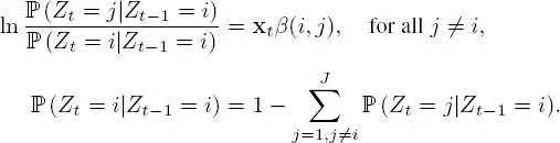

The first equation indicates that the probability of switching to a different activity j from a current activity i is connected to external conditions via a linear combination of covariates at time t . β ( i, j ) is the column vector (of dimension p ) of the coefficients corresponding to the influence of each covariate on this probability. The second equation is a constraint equation that ensures that the vector (ℙ ( Zt = 1| Zt− 1= i )) , . . . , ℙ ( Zt = J | Zt− 1= i )) is a probability vector.

It is thus possible to take account of notions such as the fact that an individual will spend a longer period of time actively foraging in a location that is rich in food sources, while in a less favorable environment, it will rapidly switch to a traveling state in order to move to a better location. The inclusion of covariates in this model makes it possible to identify environmental variables, which favor particular states.

Let us illustrate model [ 1.4] using a toy example. Consider an individual with a total of three possible behaviors. Thus, let J = 3 be the number of activities for this individual. Each of these activities is characterized by a different movement pattern: for example, a direct trajectory at high velocity, a more sinuous pattern at a lower speed, and a third, different pattern. As we have seen, these differences may be characterized using different metrics. In this example, we have chosen to model persistent velocity and turning velocity, using equations [ 1.7] and [ 1.8].

Thus, in model [ 1.4], ν 0is a probability vector of size 3, Π is a 3 × 3 matrix such that the sum of the elements in each line is equal to 1, and, for 1 ≤ j ≤ 3, distribution ( θj ) is a distribution ℕ ( μj, Σ j), where:

– μj is a vector of dimension 2 (the mean of V p and V r for activity j);

– Σj is a variance–covariance matrix (of size 2 × 2).

Using the model defined by [ 1.4], inference is used to fulfill two purposes:

– Estimation of activity: to determine the distribution of real activities given the observations, that is, for 0 ≤ t ≤ n, the distribution of the random variable Zt|Y0:n. For each time t, the estimated smoothing distribution gives the probability of being involved in each of the j activities.

– Estimation of parameters: the distribution ν0 and the transition matrix Π characterize the dynamic of activities, and the set of parameters {θj} 1 ≤ j ≤ J indicates the way in which the activity influences the distribution of observations.

In the case of unknown parameters, these two steps are carried out conjointly. Taking a frequentist approach, the EM algorithm may be used, as in section 1.2.1. Once again, it is easy to write an equation, analogous to [ 1.2], giving the full likelihood.

For this model, step E once again consists of calculating the quantity given by [ 1.4]. Again, the difficulty lies in calculating the smoothing distribution. Nevertheless, the discrete character of the hidden dynamic means that explicit calculation is possible. This is carried out iteratively using the forward–backward algorithm. The equations used in this simple and efficient algorithm can be found in Rabiner (1989).

Step M, in which the parameters are updated, is dependent on the nature of the emission distribution. In the Gaussian case, this step has an explicit expression; conversely, this is not the case when using a distribution such as von Mises.

Bayesian estimation may be applied by using Monte Carlo Markov Chain (MCMC) algorithms, which are found in programs such as Stan (Carpenter et al . 2017), Winbugs (Lunn et al . 2000) or NIMBLE (de Valpine et al . 2017).

The reconstruction of hidden activities allows us to identify homogeneous phases in behaviors, and is often of considerable interest from an ecological perspective. This hidden Markov model may thus be seen as an unsupervised segmentation/ classification model for movement.

One possibility is to reconstruct the most likely hidden activity for each time increment in turn, taking 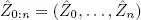such that

[1.10]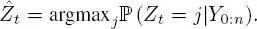

This method is known as the maximum a posteriori (MAP) method. One possible problem with the estimator [ 1.10] is that it provides no guarantee that the sequence 0:nwill be coherent with the transition matrix Π; it may give a result of t = 1 and t +1= 2 for an estimation , for example.

Using a Bayesian approach, the sampling algorithms used to estimate parameters permit the use of a joint smoothing distribution, that is, samples of Z 0:n| Y 0:ncan be obtained. Each sample produced is thus a possible sequence of activities corresponding to given observations.

Sampling across this distribution can also be carried out in conjunction with a frequentist approach, but the combinatorial level is high and the computational effort involved rapidly becomes prohibitive as n increases. Hidden activities are most commonly reconstructed using the most probable sequence of hidden states, that is, which maximizes the overall a posteriori distribution, or, more formally,

This sequence can be calculated in an efficient manner using the Viterbi algorithm, and is the version which is generally returned by libraries offering frequentist estimation. Note that the m most probable sequences can be obtained using the generalized Viterbi algorithm (Guédon 2007).