Nathalie Peyrard - Statistical Approaches for Hidden Variables in Ecology

– The emission distribution (or observation model): the observation is taken to be a random Gaussian variable centered about an affine transformation of the current position, with variance–covariance matrix Σo. The affine transformation is given by two parameters: a matrix B (of size 2 × 2) and a vector ν of dimension 2. The most common approach is to consider that ν = 0 and to take B as the identity matrix. The observation is thus presumed to be centered about the real position.

Using the model defined by [ 1.1], inference is used for two purposes:

– Estimation of positions: in this case, inference is used to determine the distribution of actual positions based on observations, that is, for 0 ≤ t ≤ n, the distribution of the random variable Zt|Y0:n. This distribution is known as the smoothing distribution.

– Estimation of parameters: to estimate the unknown parameters in the model (which, in the majority of cases, correspond to the two variance–covariance matrices, Σm and Σo).

With known parameters and for any 0 ≤ t ≤ n , the distribution of Zt | Y 0:nis Gaussian. The mean and the variance–covariance matrix of this distribution can be calculated explicitly. This step is carried out using Kalman smoothing, which will not be described in detail here; interested readers may wish to consult Tusell (2011). It is important to note that the explicit nature of this solution is exceptional in the context of latent variable models, and is a result of the Gaussian linear formulation of model [ 1.1].

In practice, the parameter θ = { μ, A, ν, B, Σ m, Σ o} is unknown. In a frequentist context, the natural aim is to identify the parameter that maximizes the likelihood associated with observations Y 0:n:

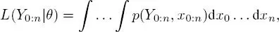
where p is a generic notation for probability density. In this case, the expression of likelihood implies the calculation of an integral in very high dimensions, as it must be integrated across all hidden states. However, given a known sequence of real positions X 0:n, we would have an explicit expression of the full log-likelihood :

[1.2]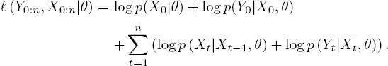

As all of the densities in this model are Gaussian, maximization of the log-likelihood would be simple. The expectation–maximization (EM) algorithm uses this full likelihood to maximize likelihood. Based on an initial parameter value θ (0), the algorithm produces a series of estimations as follows:

– Step E calculates: [1.3]

– Step M takes:

The series converges to a local maximum likelihood (Dempster et al . 1977). Equation [1.3]consists of calculating the expectation of [ 1.2] with respect to the distribution of missing data given the existing observations, that is, the distribution of X 0:n| { Y 0:n= y 0:n), using a “real” parameter The smoothing distribution for the parameter must, therefore, be calculated as part of this step; this is done using Kalman smoothing. A solution is then obtained explicitly in step M thanks to the Gaussian linear nature of the problem.

As we have seen, the reconstruction of a trajectory is reliant on the determination of a smoothing distribution, that is, for all 0 ≤ t ≤ n , the distribution of Zt | Y 0:n. Note that the inference of the real position at a time t takes account of all observations . As this distribution is Gaussian in the context of the model [ 1.1], this corresponds to calculating [ Zt | Y 0:n] and [ Zt | Y 0:n] using Kalman recursions.

The name Kalman is more often encountered in the context of Kalman filtering, rather than Kalman smoothing. In these contexts, the Kalman filter is used to determine the filter distribution , that is, the distribution of Zt | Y 0:t. It is, thus, the distribution of the position at time t on the basis of the observations up to time t .

Intuitively, smoothing gives a better estimation than filtering, as the future can be taken into account when estimating a position at time t . Using filtering, the t thposition is corrected using positions observed up until time t , while in the case of smoothing, all of the available information is taken into account. Figure 1.2, taken from Lopez et al . (2015), illustrates the advantages of smoothing. A precise, frequent recording of the movement of an elephant seal, obtained using GPS (the reference curve), is shown alongside a reconstruction of the same real trajectory obtained using Argos data, filtering and smoothing.

As we indicated earlier, an individual alternates between different activities, and these are reflected in different modes of movement. For example, an individual who is looking for food will move slowly, with frequent changes of direction as potential food sources are detected. An individual traveling back to the colony, on the other hand, will travel relatively quickly and in a relatively straight line.

Subjacent (hidden) activities may be reconstructed by analyzing a trajectory, using a model that connects activities and movement. In this case, the observations y 0:n= ( y 0 , . . . , yn ) are measures of a metric, which is presumed to be affected by an animal’s activity (typically, this metric represents speed; other examples are discussed in the following section). Taking 0 ≤ t ≤ n , zt is used to represent the unobserved activity of an individual at an instant t . This activity is encoded as an integer between 1 and J , where J is a known integer, representing the number of expected activities. Observations and hidden activities are considered as realizations of random variables. Let Z:= ( Z 0 , . . . , Zn ) be the series of hidden states (subjacent activities) and Y:= ( Y 0 , . . . , Yn ) the series of movement measurements.

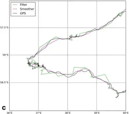
Figure 1.2. Figure extracted from Figure 4 in Lopez et al . (2015). The black line shows a precise recording of the movements of an elephant seal. The green line was obtained by filtering positions recorded using the Argos system, and the purple line shows a smoothed version of the same data. The trajectory reconstructed using smoothing corresponds more closely to the reference data than the version obtained by filtering. For a color version of this figure, see www.iste.co.uk/peyrard/ecology.zip