Nathalie Peyrard - Statistical Approaches for Hidden Variables in Ecology

McKinley, D.C., Miller-Rushing, A.J., Ballard, H.L., Bonney, R., Brown, H., Cook-Patton, S.C., Evans, D.M., French, R.A., Parrish, J.K., Phillips, T.B., Ryan, S.F., Shanley, L.A., Shirk, J.L., Stepenuck, K.F., Weltzin, J.F., Wiggins, A., Boyle, O.D., Briggs, R.D., Chapin, S.F., Hewitt, D.A., Preuss, P.W., Soukup, M.A. (2017). Citizen science can improve conservation science, natural resource management, and environmental protection. Biological Conservation , 208, 15–28.

Miller, D.A.W., Pacifici, K., Sanderlin, J.S., Reich, B.J. (2019). The recent past and promising future for data integration methods to estimate species’ distributions. Methods in Ecology and Evolution , 10(1), 22–37.

1 1 https://oliviergimenez.github.io/code_livre_variables_cachees/.

Marie-Pierre ETIENNE1 and Pierre GLOAGUEN2

1 Institut Agro, Agrocampus Ouest, CNRS, IRMAR – UMR 6625, Rennes, France

2 Paris-Saclay University, AgroParisTech, INRAE, UMR MIA-Paris, France

The study of movement in ecology has taken off in recent years, driven by questions relating to the determinisms of individual movement. Interest in the ecology of movement has been largely fueled by the emergence and development of GPS technologies over the last 20 years, helped along by the creation of numerous databases made up of individual trajectories. These observations, on fine spatial and temporal levels, can be used to study the behavior of individuals in relation to their living environment. A variety of trajectory models have been developed and applied with the aim of reconstructing these behaviors and understanding the underlying determinisms. In this chapter, we shall present two latent variable models, widely used in movement ecology for trajectory analysis. Each model corresponds to a specific objective: the reconstruction of real trajectories with the removal of any geolocation errors, and the identification of different behaviors in the course of movement.

Trajectory data are frequently marred by errors for a variety of reasons (satellite accessibility issues, geolocation errors, etc.). This results in noisy observations of the real position of the animal, which is itself unknown. The hidden variable is, therefore, the real position and the observed variable is the noisy version. In Figure 1.1, we can see that some recorded positions of a Cape dolphin, tracked using the Argos system, are actually on land – a situation which is evidently improbable. This observation almost certainly corresponds to noisy data concerning the actual position of the tracked individual.

Figure 1.1. The map at the top shows the tracking data for a male Cape dolphin (Cephalorhynchus heavisidii) in St. Helena Bay, South Africa. The coastline is shown in black, and we see that some recorded positions are actually on land. These positions are obtained using an Argos system. Figure taken from Elwen et al . (2006). Photo of a Cape dolphin by Jutta Luft, distributed under the GNU Free Documentation License. For a color version of this figure, see www.iste.co.uk/peyrard/ecology.zip

Observation errors are generally small (a few meters) in cases where positions are obtained using a GPS system on open ground and with good satellite coverage. Far larger errors may occur using other technologies, such as the Argos system (into the tens of kilometers). A hierarchical model for reconstructing real trajectories from observed trajectories is presented in section 1.2.1.

Individuals rarely move in a homogeneous manner, and different movement patterns are often observed. In Nathan et al . (2008), the authors propose a formalization of the mechanisms responsible for individual movement. Among the different aspects mentioned, the internal state of the individual and the environment in which it exists are identified as important mechanisms of movement. It seems reasonable to believe that the internal state of an individual affects its behavior, resulting in a change of movement regime.

Any study of individual movement must permit the identification of different states or activities. In this case, the hidden variable is the activity of the individual , while the observed variable is its position, or various metrics derived from this position, as we shall see later. Section 1.2.2presents a reconstruction of behavior based on movement observations, using a specific latent variable model known as a hidden Markov model.

In cases where there are errors in observed positions, data can be smoothed in order to recreate the real trajectory. To smooth errors, all collected data points are combined with a movement model in order to “straighten out” outlying observations and thus correct positioning errors.

Different ways of taking account of observation errors in movement models have been discussed at length in the literature (Freitas et al . 2008; Johnson et al . 2008; Patterson et al . 2010). For initial, simple trajectory reconstructions, however, a linear Gaussian hierarchical model can be used as a first data exploration. This approach draws on the notion that the observed position is a noisy version of the real position, and that the noise around this position is Gaussian. In formal terms, take n noisy observations, y 0:n= ( y 0 , . . . , yn ), of an animal’s position. Generally speaking (and throughout this chapter), we presume that each observed position is a vector of ℝ 2. These observations are presumed to be realizations of random variables Y 0:n, the distribution of which depends on the real position of the animal. Moreover, the real position of an animal at a given instant (unknown) is dependent on its real position for the previous instant (also unknown). In formal terms, these positions themselves can be seen as a sequence of non-independent random variables, noted Z 0:n= ( Z 0 , . . . Zn ), with values in ℝ 2.

We consider that all of these random variables obey the following hierarchical model:

[1.1]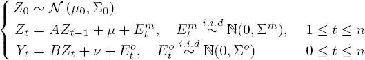

From top to bottom, these three equations define:

– The initial distribution: the a priori initial position of the individual. In this case, we have a normal distribution (in dimension 2) about an initial position μ0, with a variance–covariance matrix Σ0.

– The transition distribution (or dynamic model): in this case, a model of the individual’s movement. We consider that the current position is given by a random Gaussian variable, centered about an affine transformation of the previous position, with a variance–covariance matrix Σm. The affine transformation is obtained from two parameters: a matrix A (of size 2 × 2) and a vector μ of dimension 2. The most common approach is to consider that μ = 0 and to take A as the identity matrix. The resulting model is a random walk.