Nathalie Peyrard - Statistical Approaches for Hidden Variables in Ecology

Using a classic activity reconstruction approach, the sequence Zis modeled by a Markov chain, that is, the series of random variables Zt verifies the Markov property; in other terms, for any series of integers z 0:twith values in { 1 , . . . , J } i +1:

Furthermore, if we consider that this probability of transition is independent of the instant t , the Markov chain is said to be homogeneous 1.

The model draws on the idea that the distribution of Yt is dependent on the activity. The modeler must, therefore, specify the distribution of Yt |{ Zt = j }. This specification is generally carried out using a parametric distribution (typically a normal distribution). Activity identification is based on the ways in which the parameters of this distribution change (the mean and variance change as the activity changes).

The full model is formulated as follows:

[1.4]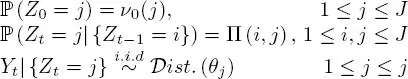

From top to bottom, these three equations define:

– The initial distribution: this the probability distribution for the first activity, and is thus a vector of probabilities ν0 = (ν0(1), . . . , ν0(J)). In the common case where only one trajectory is observed, the initial distribution is taken to be known, or equal to a uniform distribution over {1, . . . , J}.

– The transition distribution: in the case of a homogeneous Markov chain, the transition distribution is fully characterized by the matrix Π, of size J × J, of which each line is a probability vector.

– The emission distribution: the observation is taken to be a random variable, the distribution of which depends, via these parameters, on the activity. The nature of the distribution depends on the nature of the observations. Note that observations are considered to be independent, conditionally to Z.

This model is shown in the graphical form in Figure 1.3.

This general framework offers many possibilities in terms of modeling. The subjacent activity may influence different aspects of the trajectory. For example, the trajectory of an individual looking for food will include multiple changes in direction. On the other hand, when an individual is traveling, in the context of migration, for example, its trajectory tends to be relatively straight with only minor changes in direction. In this example, changes in direction are strong activity markers.

Most of the metrics encountered in existing literature are based on the speed and direction of the animal in question.

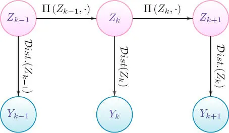
Figure 1.3. Graphical model. For a color version of this figure, see www.iste.co.uk/peyrard/ecology.zip

Starting from the positions { Pt } t≥ 0(with values in ℝ 2obtained at times 0 , Δ , 2Δ , . . . ), the process of speeds { Vt } t≥ 1is defined by

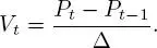
From these speeds, we can define the direction { ψt } t≥ 0(with values in [ −π, π [) as the angle between Vt and a reference vector (typically the vector (1, 0) pointing east). From these metrics, we deduce step length (or scalar speed) processes, denoted as { Lt } t≥ 1, and turning angles, denoted as{ φt } t≥ 1(with values in ] − π, π ] using the convention φ 1= 0) as follows:

[1.5]

[1.6]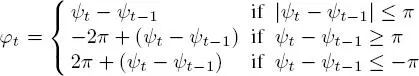

The step length and turning angle metrics were the first to be used in behavior, or activity, analysis based on HMMs (Morales et al . 2004) and have been widely used (Patterson et al . 2008). In this way, we obtain the model illustrated in Figure 1.3, where Yt is a bivariate vector of coordinates ( Lt, φt ) (often considered to be independent). One drawback to this method is the need to define an emission distribution, which is compatible with angles in order to model ( φt ). In practice, Von Mises (Jammalamadaka and Sengupta 2001) or Wrapped Cauchy distributions are the most widely used.

A different set of equivalent metrics may be used in order to avoid working with circular distributions, as proposed in Gurarie et al . (2009) and Gloaguen et al . (2015); these are persistence velocity and turning velocity

[1.7]

[1.8]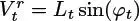

An observation Yt is thus a vector made up of these two components. As these components are signed, it is logical to model Yt using a bivariate normal distributions. Where relevant, this model allows the introduction of a dependency relationship between the two movement components, something which is difficult to achieve when selecting a couple ( Lt, φt ).

Ecological expertise concerning the effects of different activities on movement can also contribute to the choice of an appropriate metric. In the case study presented at the end of this chapter, the two classic metrics were used to illustrate the difference between the two approaches, in terms of both results and practical implementation.

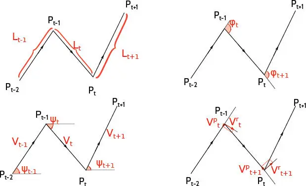
Figure 1.4. Illustration of the quantities present in equations [ 1.5] – [ 1.8] . Pt denotes the successive positions occupied by the tracked individual. The series of speed vectors denoted as ( Vt ) and ( Lt ) denotes step length as defined by equation [ 1.5] . The series of directions is denoted as (Ψ t) , while ( φt ) is the series of turning angles as defined by equation [ 1.6] . For a color version of this figure, see www.iste.co.uk/peyrard/ecology.zip