Nathalie Peyrard - Statistical Approaches for Hidden Variables in Ecology

– Bivariate velocity change metric (Gurarie et al. 2009): the emission distributions in this case are two independent normal distributions. This model will be labeled bivariate speed in our figures.

These models do not include any covariates, and the initial distribution will not be estimated. Each model is made up of 18 parameters (12 emission distribution parameters and six transition matrix parameters). Iterative optimization applied to a space of this type (such as the EM algorithm) may be affected by the chosen starting point. In both cases, the choice of a suitable starting point for the algorithm is crucial. One relatively generic approach involves a classification of k -averages (for the selected metrics). This rapid classification can be used to identify plausible parameters for different regimes; nevertheless, it is still important to ensure that the result obtained from the algorithm has not been affected by the choice of starting point.

In the two packages used here, the parameters of the HMM are estimated using maximum likelihood, and the sequence of most probable hidden states is retraced using a Viterbi algorithm.

The hidden states in this model characterize the distribution of speeds and turning angles. In terms of trajectories, this implies that a hidden state characterizes a segment between two positions (10 s apart, in this case). States on the trajectory are thus represented on these segments. In this unsupervised classification approach, the labels assigned to hidden states (interpreted as behaviors) are arbitrary, and each state must be characterized a posteriori . For ease of interpretation, we have chosen to categorize three states according to the average observed speed. State 1 corresponds to the activity with the lowest average speed, while state 3 corresponds to the fastest average speed.

Figure 1.8shows the behaviors identified by inference along trajectories for the two models used here.

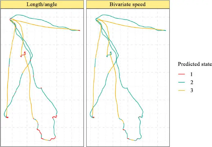
Figure 1.8. Representation of states along trajectories estimated using two different models. States are classified in order of relative speed, from slowest (1) to fastest (3). For a color version of this figure, see www.iste.co.uk/peyrard/ecology.zip

It is clear from the figure that the two models result in different nuances in the trajectories.

– Using the length/angle metric, three states are clearly visible, notably a “slow” state that characterizes the erratic phases of the trajectory. An intermediate state (2) characterizes trajectories of medium speed and a medium level of eraticness, while the third state reflects fast, direct movement.

– Using the bivariate velocity, metric, a similar third state is obtained, but there are significant differences in terms of the distinction between the first two states. In the first state, the bird appears to be “drifting”, at slow speeds with little variation. The second state appears to characterize all movement during which the bird is not resting, with a high level of variation in terms of speed.

This initial interpretation can be extended by analyzing the distribution of step length and turning angles by state 3( Figure 1.9).

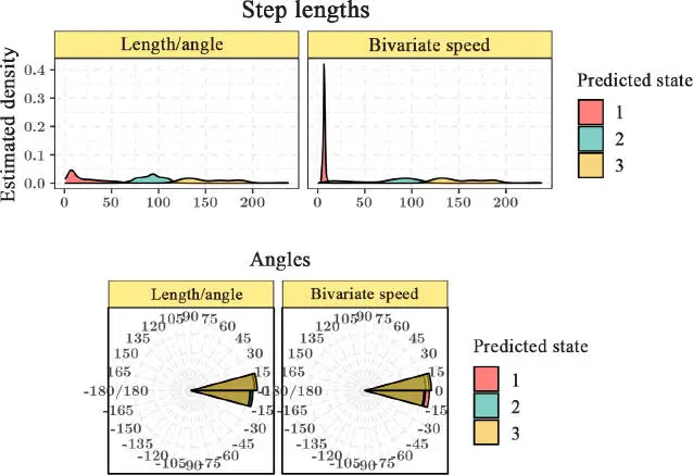
Figure 1.9. Distribution of our chosen metrics for the states estimated using our two models. For a color version of this figure, see www.iste.co.uk/peyrard/ecology.zip

It is immediately evident that the distinction between states is not based on the distribution of turning angles in either model. The influence of the step length distribution is much clearer.

We see that, for the length/angle metric, the slow state corresponds to movements of between 0 and 50 m; using the bivariate velocity metric, this same state corresponds to movement over very short distances (of the order of 5 m). Consequently, state 2 covers different speed intervals; using the first metric, this state corresponds to step lengths of 60–120 m, whereas for the second metric, this state corresponds to step lengths of 0–100 m, including much shorter distances (of around 20 m). Conversely, step 3 (rapid movement) corresponds to similar movement patterns in both metrics.

This distinction can also be seen in the table of state contingencies by metric ( Figure 1.10).

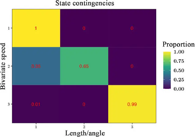
Figure 1.10. Contingencies of estimated states for our two models. For a color version of this figure, see www.iste.co.uk/peyrard/ecology.zip

Once again, we see that state 1 of the bivariate velocity metric falls within state 1 of the Length/Angle metric; similarly, the third states of the two metrics correspond. The metrics differ in the way in which state 2 is characterized: state 2 of the Bivariate Velocity metric corresponds to a combination of states 1 and 2 of the Length/Angle metric.

These differences are not surprising, given the differences between the underlying metrics. We have chosen to highlight this difference here for illustrative purposes, but it should be noted that, for a four-state model, the disparities are much smaller.

In this context, the characterization of states and the choice of the “best” model is based on interpretation, drawing on biological knowledge of the species in question. As is often the case, this unsupervised approach is most suitable for exploratory purposes, and should be interpreted in light of the ecological context.

One advantage of the probabilistic version of supervised classification is the fact that the uncertainty of classification can be quantified. In this case, we can consider the evolution of the probability of being in state 1 or state 2 over time. Figure 1.11illustrates this evolution for one of the three boobies.

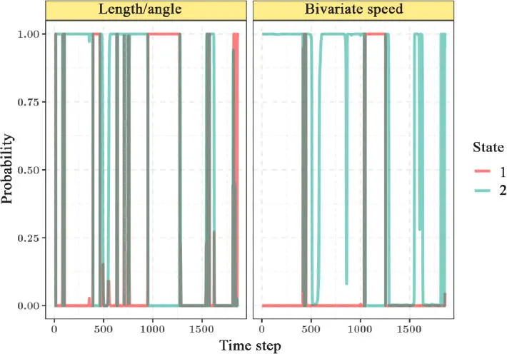
Figure 1.11. Evolution of the probability of being in state 1 or state 2 over time, by model. For a color version of this figure, see www.iste.co.uk/peyrard/ecology.zip

We see that the level of uncertainty in terms of state classification is very low, as the separation of distributions in each state is clear.

Our model may be developed further by adding a covariate, in this case the bird’s distance from the nest. We wish to determine whether changes in activity are correlated with distance from the nest. Using the formulation given in equation [1.9], we write:

where dt is the distance from the nest at time t . A quadratic component has been added to take account of the potentially variable character of the relation between the probability of transition and the covariate.