Applications of Polymer Nanofibers

The book addresses the basic science behind fabrication and nanofiber characterization with a clear emphasis on practical aspects of electrospinning. An attempt has been made to compile the more recent information and cover the different application areas where novel uses will be found for nanofiber materials.

Anthony L. Andrady

Saad A. Khan

Department of Chemical and Biomolecular Engineering

North Carolina State University

1 1Silk threads from spider species Nephila clavipes Vehoff, T., Glisović, A., Schollmeyer, H., Zippelius, A. et al. (2007). Mechanical properties of spider dragline silk: humidity, hysteresis, and relaxation. Biophysical Journal 93 (12): 4425–4432.

Christina Tang1, Shani L. Levit1, Kathleen F. Swana2, Breland T. Thornton1, Jessica L. Barlow1, and Arzan C. Dotivala1

1Department of Chemical and Life Science Engineering, Virginia Commonwealth University, Richmond, VA, USA

2U.S. Army Combat Capabilities Development Command Soldier Center, Natick, MA, USA

Electrospinning has been widely used to produce nonwoven nanofibers for applications in biomaterials, energy materials, composites, catalysis, and sensors (Agarwal et al. 2008, 2009; Ahmed et al. 2014; Cavaliere et al. 2011; Chigome and Torto 2011; Ma et al. 2014; Mao et al. 2013; Yoon et al. 2008; Thavasi et al. 2008). On a bench scale, it is a simple, inexpensive process. To generate nanofibers by electrospinning, an electric potential is applied between a capillary containing a polymer solution or melt and a grounded collector ( Figure 1.1). The applied electric field leads to free charge accumulation at the liquid‐air interface and electrostatic stress. When the electrostatic stress overcomes surface tension, the free surface deforms into a “Taylor cone.” Balancing the applied flow rate and voltage results in a continuous fluid jet from the tip of the cone. As the jet travels to the collector, it typically undergoes nonaxisymmetric instabilities such as bending and branching leading to extreme stretching. As the fluid jet is stretched, the solvent rapidly evaporates to form the polymer fibers that are deposited onto a grounded target (Reneker and Chun 1996; Helgeson et al. 2008; Rutledge and Fridrikh 2007; Thompson et al. 2007; Teo and Ramakrishna 2006; Li and Xia 2004). As a complex electrohydrodynamic process, the final fiber and mat/membrane properties depend on process parameters by process parameters, setup parameters, and solution properties.

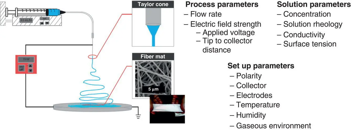
Figure 1.1 Schematic of conventional electrospinning setup and overview of process, setup, and solution parameters that affect fiber and mat properties.

Source: Photograph of mat reprinted from Dror et al. (2008). Copyright (2008). American Chemical Society.

Electrospun fibers from 30 nm to 10 μm in diameter have been reported (Greiner and Wendorff 2007). Despite its widespread use, electrospinning of new materials is typically done ad hoc varying polymer concentration and process variables. Although the nanofiber properties, namely fiber diameter, could be ideally controlled by varying the process parameters, precise control over the fiber diameter remains a technical bottleneck. The effect of process variables on fiber characteristics has been widely examined theoretically and experimentally.

To avoid the cost and time of experimental trial and error, modeling and theoretical analysis have been applied to predict how process parameters affect fiber diameter. Reneker and coworkers have developed a theoretical model based on simulating jet flow as bead‐springs. Their model describes the entire electrospinning process and accounts for solution viscoelasticity, electric forces, solvent evaporation and solidification, surface tension, and jet–jet interactions. Performing sensitivity analysis of 13 model input parameters, they determined that initial jet radius, tip‐to‐collector distance, volumetric charge density, and solution rheology, i.e. relaxation time and elongational viscosity, had strong effect on final fiber size. Initial polymer concentration, perturbation frequency, solvent vapor pressure, solution density, and electric potential had a moderate effect, whereas vapor diffusivity, relative humidity, and surface tension had minor effects on fiber diameter (Thompson et al. 2007).

Using a simple analytical model focusing on the whipping of the jet treats the jet as a slender viscous object. Rutledge and coworkers assume that the final fiber diameter is dictated by an equilibrium between Coulombic charge repulsion on the surface of the jet and the surface tension of the liquid jet. The model predicts that terminal jet radius ( r j)

(1.1)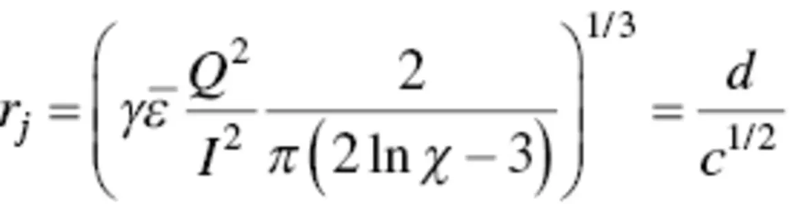

where Q is the volumetric flow rate, I is the electric current, γ is the surface tension, is the dielectric constant of the outside medium (typically air), and χ is the dimensionless wavelength of the instability of the normal displacement. The fiber diameter ( d ) is related to the terminal jet radius and the polymer concentration, c . When compared to experimental results, the model accurately predicted the diameter of polyethylene oxide (PEO) fibers (within 10%) and polyacrylonitrile fibers (within 20%). The theory overpredicted stretching for polycaprolactone fibers, which had relatively low conductivity and high solvent volatility (Fridrikh et al. 2003).

Recently, Stepanyan and coworkers developed an electrohydrodynamic model of the jet elongation in which kinetics of elongation and evaporation govern the nanofiber diameter. Using the timescale of elongation to nondimensionalize the force balance, the timescale of solvent evaporation, and concentration‐dependent material functions (e.g. relaxation time), they predict the scaling relationship for the final fiber radius ( r f) is

(1.2)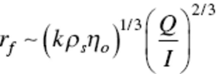

where k is the solvent evaporation rate, ρ sis the solution density, η ois the solution viscosity, Q is the volumetric flow rate, and I is the electric current. The result for Eq. (1.2)reduces to Eq. (1.1)in the limit of very slow evaporation. The viscosity dependence, η o 1/3, and ( Q/I ) 2/3agree with experimental results. Using polyvinylpyrrolidone (PVP) in various alcohol solutions as well as polyamide/polyacrylonitrile in dimethylformamide (DMF) solutions, the fiber diameter was experimentally observed to scale with the evaporation rate, k , to the 1/3 power (Stepanyan et al. 2014, 2016).

The current in electrospinning ( I ) and the volumetric charge density ( Q/I ) is commonly used in modeling and theoretical approaches. Experimental investigations by Yarin and coworkers determined that