Ted Kwartler - Sports Analytics in Practice with R

Now that the data has been modified, it will be readily accepted by the ` ggplot` function. Instead of the previous ` qplot` function, now the more expansive ` ggplot` function is called. The first parameter is the ` data` object. The next parameter is the ` mapping` aesthetics. This is a multi-part input declared with yet another function ` aes`. Within the ` aes` function, the column names to be plotted are defined. Specifically, the x -axis column name, ` stat`, followed by the y -axis column name ` player`, and finally the fill value which corresponds to the ` value` column. Thus, the visual is set up so that player statistics are arranged on the x -axis, individual players will be a single row along the y -axis, and the color intensity will be scaled by the players corresponding statistical value. Once the base layer plot has been defined, another layer is added with the ` +` sign to declare the type of plot needed. In this case, the heatmap is called using ` geom_tile`. In subsequent chapters, additional visuals are illustrated including ggplot2 and more dynamic interactive graphics. Since this text requires gray-scale graphics, another layer is added to define the color intensity between ` lightgrey` and ` black`. Finally, another layer is added to retitle the x -axis label as “Scoring Statistics” encased in quotes because it is a label not an object or column name. For simplicity, this is captured in an object called ` heatPlot`.

heatPlot <- ggplot(data = nbaDataLong, mapping = aes(x = stat, y = player, fill = value)) + geom_tile() + scale_fill_gradient(low="lightgrey", high="black") + xlab(label = "Scoring Statistics")

Although calling ` heatPlot` now in the console will create the visual, some additional layers can be added. First, a predefined theme for Highcharts is added, just as before using ` theme_hc`. Next, a chart title is declared with ` ggtitle` along with the quoted “Dallas Team Offensive Stats.” Lastly, a ` theme` is appended as the final layer that simply removed the legend altogether. Now when the ` heatPlot` object is called, a clean, visually compelling plot is created that clearly shows the most offensively productive player for the three statistics on the team. Additionally, other player’s strengths in these statistics are easily understood because their sections are darker compared to teammates. Conversely weaker players in these stats have a lighter color. These facts are more quickly understood in a visual compared to reviewing a table of player data. The result of the ` heatPlot` object is shown in Figure 1.9.

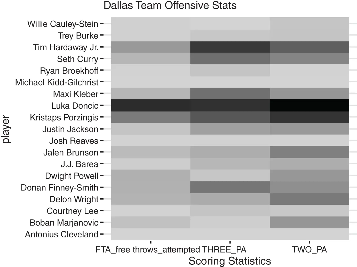
Figure 1.9 The Dallas team statistics represented in a heatmap illustrating the most impactful players among these statistics in the 2019–2020 regular NBA season.

heatPlot <- heatPlot + theme_hc() + ggtitle('Dallas Team Offensive Stats') + theme(legend.position = "none")

There are multiple ways to extend the lessons of this chapter to improve R coding fluency. For example, the data itself can be explored further or subset by position. Additional visualizations are also possible although many of these topics are covered in subsequent chapters with expanded explanations.

In the end, R should be known as a scripting language. It is not a “low level language” like Java where the code itself is executed directly on the hardware such as a central processing unit, CPU. As a scripting language R cannot be compiled into an executable standalone program. As a result, R has some constraints, in that it is slower than other languages like Java and building a standalone application is not possible. However, the benefit is that R is capable of executing multiple operations borrowing from languages as needed and it well suited to statistical tasks. For example, operations in machine learning like Random Forest are called with R functions yet executed in Fortran. Still other functions borrow from C, SQL, Weka, and so on. This diversity makes the functionality high because the functional tool set is vast but with so much going on under the hood, R can be slow. Another drawback to R is that objects are stored in active memory. As a result, data objects are limited by the amount of RAM on your laptop or R-Studio server. For many data tasks this is not a problem especially as you transition to scalable cloud servers. In fact, in this text, all the data tasks and computation are relatively small. Constraints start to exist after loading millions of rows and columns in a data frame or when doing computationally complex calculations as is the case with Depp Neural Networks. However, this book is focused on sports analytics rather than big data or machine learning exclusively. Thus, these drawbacks to the R language will not be an issue.

Besides the ability to execute functions drawing from across multiple specialized languages R has other positive benefits. For example, R has a well-developed support community. Often when you are presented with an error or unknown operation, a simple online search will identify the solution. Additionally, R is optimized for statistics. Although python, a competing and more-diverse language has similar functionality, there are still differences between the two languages. For example, some machine learning-tuning parameters are better executed in R, the simple creation of dynamic HTML-based dashboards is easier or file formats like “fst” are more enhanced within R. Given that R is not picky about spacing and indentation, it is an excellent language for the novice programming. As you scale your learning in analytics and coding, you will likely want to add to your language toolkit.

1 How is an IDE different than a coding language?

2 Describe the difference between a vector and a data frame or matrix?What is the difference between a data frame and matrix?

3 Construct a vector called `position` where the values are:“Center,” “Forward,” “Guard,” “Forward,” “Forward,” and “Guard.”Change the object type from character as it was constructed into a factor.Tabulate the `position` factor object using `table` in a new object called `tallyPosition`.Use a new function to quickly create a bar plot of the results. To do so, apply `barplot` on the ` tallyPosition` object.

4 Load ` library(RCurl) ` then create an object called “bostonStats” by loading the file here: https://raw.githubusercontent.com/kwartler/Practical_Sports_Analytics/main/C1_Data/2019-2020%20Boston%20Player%20Stats.csvHow many rows does this data frame have?How many columns does this data frame have?Examine the last 4 rows of the data programmatically? What player is listed as the fourth from the bottom?Using either indexing or column name, get summary statistics for the `GP_games_played` column. What is the third quartile of this statistic?

5 Load ` library(ggplot2) ` then create a quick plot of ` STEALS_PER_GAME` and ` TURNOVERS_PER_GAME`. Does there appear to be a relationship to the syle of play for strong defense and turnovers?

6 Load `library(tidyr)`, then create a heatmap of the Boston team data using ` REBOUNDS_PER_GAME`, ` ASSISTS_PER_GAME`, ` STEALS_PER_GAME`, and `BLOCKS_PER_GAME` by ` ï.PLAYER`Create a small data frame renaming the player column.Pivot the data frame.Create a `ggplot` visual with the pivoted data where` aes(x = stat, y = player, fill = value)`The chart type is `geom_tile()`The color intensity scales from “lightgreen” to “darkred”The x-axis label “Basketball Statistics”