Ted Kwartler - Sports Analytics in Practice with R

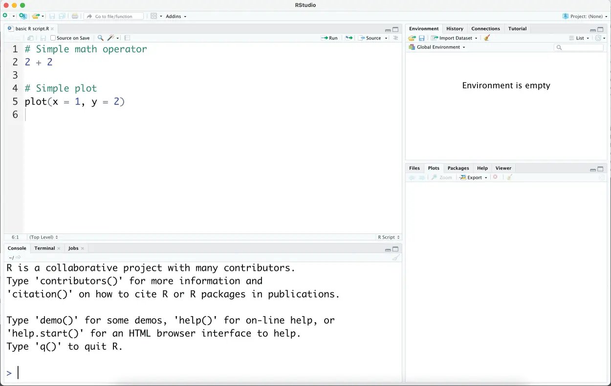
Figure 1.3 The upper left R script with basic commands and comments.

Of particular note in the script shown in Figure 1.3 are two comments and two code examples. A comment begins with a ` #`. This tells R to ignore everything on that line. As you begin your learning journey programming in R, it is a best practice to add comments to remind yourself the nuances of the code to be executed. Thus, feel free to make a copy of any scripts throughout the book, add comments, and save for yourself.

The first code to be executed, beginning on a non-commented line, is a simple arithmetic operation shown below.

2 + 2

Since this is in a script, it will not be run until you declare it within the console. Further, as you can guess the operation ` 2 + 2` has a single result ` 4`. An easy way to run the script is to place your cursor on the line you want to execute and click the “run” icon on the upper right-hand side of the script. When this is done the code is transferred to the console and executed, returning the single answer as expected. Figure 1.4 illustrates the transfer between script and console.

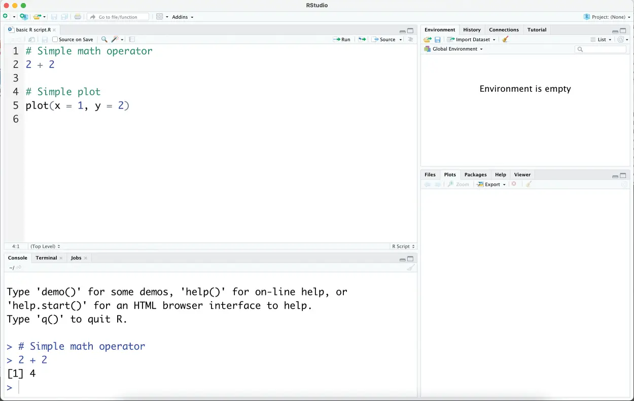
Figure 1.4 Showing the code execution on line 2 of the script being transferred to the console where the result 4 is printed.

Next, let’s execute another command which will illustrate another pane of the IDE. If your cursor is on line 5 of the R script, ` plot(x = 1, y = 2)` and you click the “run” icon you will now see a simple scatter plot visual appear in the lower right utility pane titled “Plots.” Each tab of the utility pane is described below:

Files—This is a file navigation view, where you can review folders and files to be used in analysis or saved to disk.

Plots—For reviewing any static visualizations the R code creates. This pane can also be used for resizing the image using a graphical user interface (GUI) and saving the plots to disk.

Packages—Since R needs to be specialized for a particular task, this pane lists your local package library with official documentation and accompanying examples, vignettes, and tutorials.

Help—Provides various resources for obtaining help with R and its many tasks.

Viewer—This pane allows you to view the small webpages and dynamic interactive plots which R can create.

Figure 1.5 shows the result of a basic, yet not visually appealing scatter plot with a single point. Rest assured the plots throughout the book are more compelling than this simplistic example. The x , y coordinate points are defined in code as ` x = 1` and ` y = 2`.

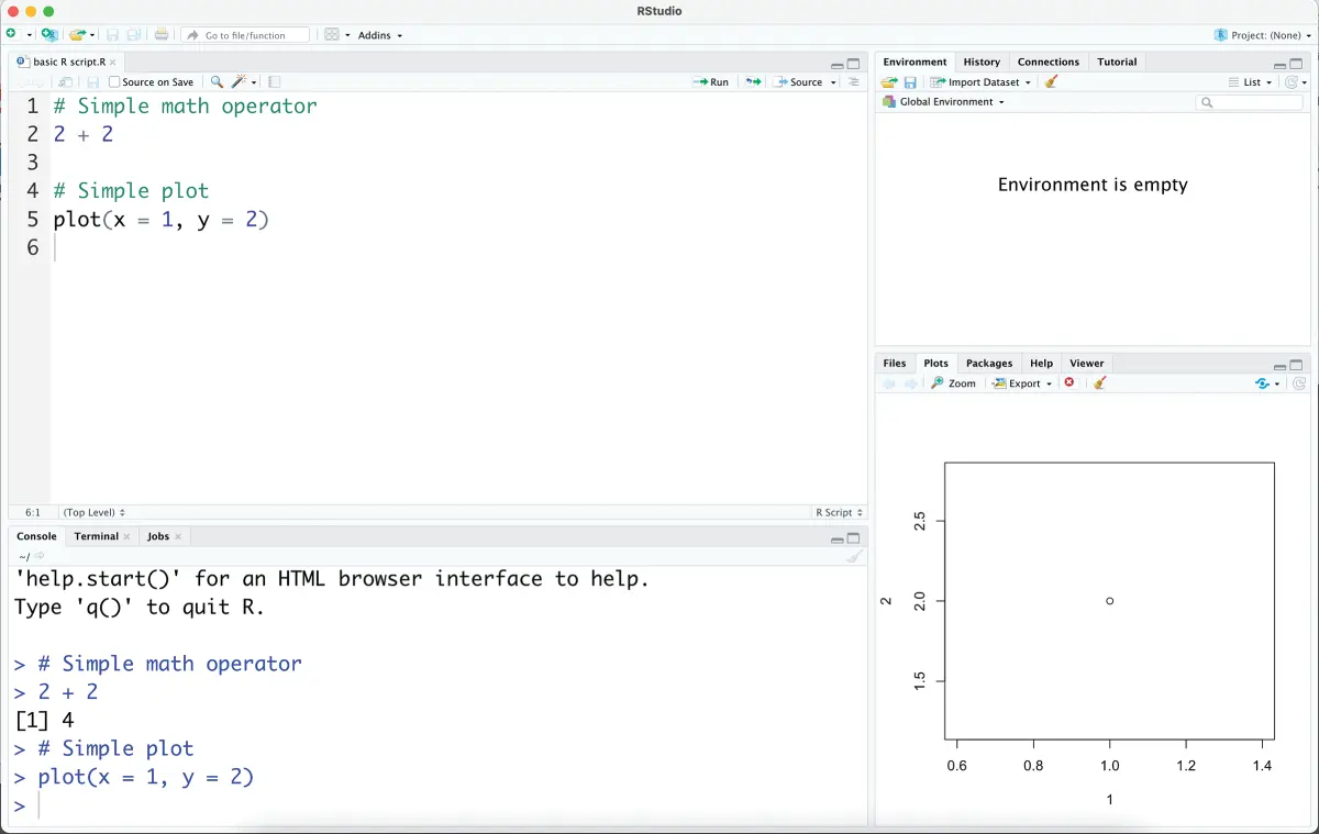
Figure 1.5 The basic scatter plot is instantiated in the lower right, “Plots” plane.

Next, let’s focus on the remaining upper right pane of the IDE. The primary tab of interest is the “Environment” tab. R works by creating objects which are stored data objects. When an object is created, it is held in active memory, your computer’s RAM. Any active objects in your R session will be shown in the “Environment” tab in the upper right. Add the following code in the script (upper left) pane, then click “run” to instantiate an object in your environment. Notice the first bit follows a ` #` so the non-code comment “Create an object” acts as a signpost for you while the next line actually creates the object. Specifically, the object name is ` xVal` and it is declared have a value of ` 1`. Moreover, the declaration of the object name to value is done with the assignment operate ` <-`. In the R language you can also use an equal sign for the object name assignment. However, most R style guides use the ` <-` operator and this book follows that direction.

# Create an object xVal <- 1

When run the upper right environment tab will now show an object, ` xVal`, that is held in memory for use later in the script. Of course, these objects can become much more complex than a single value. Next add more code to your script utilizing the ` xVal` object rather than declaring the value explicitly. The following code can be added to your script and then run to recreate the simple scatter plot from before. The difference is that R has substituted the ` x = xVal` input to ` x = 1` since that is the object’s actual value. The only difference in the plots is that the second one has a different x -axis title because the value was derived from the object name. Figure 1.6 now shows the additional code chunks, the new object in the environment, and the recreated plot in the utility pane.

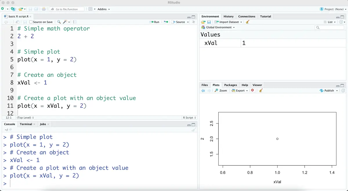
Figure 1.6 The renewed plot with an R object in the environment.

# Create a plot with an object value plot(x = xVal, y = 2)

The basic functionality of R is underpinned by functions and objects. Each package that specializes R comes with a set of functions usually coordinated for a particular task like data manipulation, obtaining sports data or similar. Functions accept inputs, including objects, and manipulate the inputs most often to create new objects or to overwrite and replace existing objects. For example, the following code creates a new object ` newObj` using the assignment operator and on the right-hand side employs a base-R function. Base-R functions do not require any libraries to be loaded, so there is no need to specialize the R environment for a particular task. The ` newObj` variable is declared as a result of a function ` round` with two input parameters. The first parameter accepts the number to be rounded, ` 1.23`. The second parameter ` digits = 0` is a tuning parameter which changes the behavior of the ` round` function declaring the number of decimals to round the input to. Thus, when you add the following code to the script and then execute it in the console, the resulting ` newObj` variable has a corresponding value of 1. As before, the ` newObj` object will be stored actively and shown in the “Environment” tab. Keep in mind the inputs themselves can be objects not just declared values. As a result of this behavior, scripts manipulate objects and often pass them to another function later in the script.

# Create a new object with a function newObj <- round(1.23, digits = 0)

This book will illustrate many functions both in base-R and within specialized packages applied in a sports context. R has many tens of thousands of packages with corresponding functions. Often the rest of this book will defer to base-R functions in an effort for standardization, stability, and ease of understanding rather than utilize an esoteric package. This is a deliberate choice to improve conceptual understanding but does leave room for code optimization and improvement.

There are additional intermediate programming operators that are employed in this book. In fact, there are multiple types of logical and arithmetic operators but for the most part the scripts in this book are focused on one use case at a time, with linear thinking, so you can focus on the concepts and applications more so than concise code. However, Table 1.1describes the three control flow operators used in the book with a code example for you to try in your script and console. Within the FOR loop, a set of code is run repeatedly with a variable that changes each time through. For the latter two, the IF and IFELSE control flows, a logical statement is evaluated and controls the code’s behavior. If the statement is run and returns TRUE, then the code is executed otherwise it is ignored.