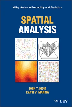
Kanti V. Mardia - Spatial Analysis

We have had helpful discussions with many participants at the LASR workshops and with colleagues and students about the material in the book. These include Robert Adler, Francisco Alonso, Jose Angulo, Robert Aykroyd, Andrew Baczkowski, Noel Cressie, Sourish Das, Pierre Delfiner, Peter Diggle, Peter Dowd, Ian Dryden, Alan Gelfand, Christine Gill, Chris Glasbey, Arnaldo Goitía, Colin Goodall, Peter Green, Ulf Grenander, Luigi Ippoliti, Anil Jain, Giovanna Jona Lasinio, André Journel, Freddie Kalaitzis, David Kendall, Danie Krige, Neil Lawrence, Toby Lewis, John Little, Roger Marshall, Georges Matheron, Lutz Mattner, Charles Meyer, Michael Miller, Mohsen Mohammadzadeh, Debashis Mondal, Richard Morris, Ali Mosammam, Nitis Mukhopadhyay, Keith Ord, E Pardo‐Igúzquiza, Anna Persson, Sophia Rabe, Ed Redfern, Allen Royale, Sujit Sahu, Paul Sampson, Bernard Silverman, Nozer Singpurwalla, Paul Switzer, Charles Taylor, D. Vere‐Jones, Alan Watkins, Geof Watson, Chris Wikle, Alan Wilson, and Jim Zidek.

John is grateful to his wife Sue for her support in the writing of this book, especially with the challenges of the Covid pandemic. Kanti would like to thank the Leverhulme Trust for an Emeritus Fellowship and Anna Grundy of the Trust for simplifying the administration process. Finally, he would like to express his sincere gratitude to his wife and his family for continuous love, support and compassion during his research writings such as this monograph.

We would be pleased to hear about any typographical or other errors in the text.

30 June 2021

John T. Kent

Kanti V. Mardia

Here is a list of some of the key notations and terminology used in the book.

and denote the real numbers and integers.

For a dimension , a site is a location or . The elements or components of a site are written using square bracketsNote is not in bold face.

A random field is synonymous with a stochastic process. A random field on is written as , using function notation. A random field on the lattice is written as , using subscript notation. A random field is often assumed to be a Gaussian process (GP).

The mean function and covariance function are written as and covariance function . In the stationary case, is constant and depends only on the lag . In the lattice case, use subscripts, e.g. .

A stationary covariance function can be written as a product of a marginal variance σ2 and an autocorrelation function ρ(h).

An intrinsic random field extends the idea of a stationary random field. Write for an intrinsic random field of order (IRF‐) with intrinsic covariance function . For an intrinsic random field of order 0 (IRF‐0), the semivariogram is given by . A registered version of an intrinsic random field is denoted .

For a stationary model, a scheme is a parameterized family of covariance functions. For an intrinsic model, a scheme is a parameterized family of intrinsic covariance functions (or equivalently for an IRF‐0 model, a parameterized family of semivariograms).

A nugget effect refers to observations from a random field subject to measurement error, with variance typically denoted .

The vector of covariance parameters for a stationary or intrinsic model, possibly including a nugget effect, is denoted and can be partitioned as in terms of an overall scale parameter and the remaining parameters.

Spaces of polynomials in (Section 3.4):– : Space of homogeneous polynomials of degree , with dimension denoted – : Space of all polynomials of degree in , with dimension denoted .

denotes the isotropic self‐similar intrinsic random field of index and with drift space (Section 3.10). The intrinsic covariance function is denoted and spectral density is denoted .

Most of the book is concerned with ordinary random fields. There are also generalized random fields indexed by functions rather than sites and written as with covariance functional .

The surface area of the unit sphere in is denoted .

denotes a domain of sites in or . The notation encompasses several possibilities, including the following:– An open subset , e.g. – A finite collection of sites in or – The infinite lattice – A finite rectangular lattice in ,with dimension vector and of size . In the lattice case, sites in can be denoted using letters such as to emphasize the link to the continuous case, or using letters such as to emphasize the fact that the components are integers.For a finite domain, the notation stands for the number of sites in .

Frequencies in the Fourier domain are denoted .

Vectors indexing data are treated as column vectors and are written as in bold lowercase letters, with the components indicated by subscripts. The transpose of is denoted . This subscript convention is typical in multivariate analysis. Note the difference from the convention for sites and frequencies .

Random vectors, e.g., or are written in bold letters, with the components indicated by subscripts. In particular, upper case is used when the distinction between a random quantity and its possible values needs emphasis.

Matrices are written using nonbold uppercase letters, e.g. and , with the elements of written as or as . The two notations are synonymous. The columns of are written using bracketed subscripts, . For a square matrix, the determinant is denoted by either or ; the notation should not be confused with , the size of a domain described above.

If and are sites, then is the inner product and is the squared Euclidean norm.

Modulo notation (for numbers) and (for vectors) (Section A.1)

Check and convolution notation. If is a function of , let . Thenand the latter is symmetric in .

The Kronecker delta and Dirac delta functions are denoted and , respectively.

. A finite symmetric neighborhood of the origin in . The augmented neighborhood includes the origin. Half of the neighborhood is denoted (Section 4.4).

. A half‐space in , especially the lexicographic half‐space (Section 4.8). Related ideas are the weak past and quadrant past (Section 4.8), and the partial past (Section 5.9).

Kriging is essentially prediction for random fields. It comes in various forms including simple kriging, ordinary kriging, universal kriging, and Bayesian kriging. In each case, there is a kriging predictor at every site, which depends on the data through a kriging vector. Combining the kriging predictor for all sites yields a kriging surface. The kriging variance describes the accuracy of the predictor at each site. Tables 7.1 and 7.2 set out the notation for kriging and Table 7.3 provides a comparison with some related notation used in machine learning.

The transfer covariance matrix and transfer drift matrix are used to construct the kriging predictor (Section 7.6).

Bordered covariance matrix. This is an matrix, Section 7.6.4, also used to construct the kriging predictor.

Autoregression (AR) and related spatial models come in various forms in Chapter 4including:– MA: Moving average (Section 4.3)– SAR: Simultaneous autoregression (Section 4.5)– CAR: Conditional autoregression (Section 4.6)– ICAR: Intrinsic CAR (Section 4.6.3)– QICAR: Quasi‐intrinsic CAR (Section 4.6.3)– UAR: Unilateral autoregression (Section 4.8.2)– QAR: Quadrant unilateral autoregression (Section 4.8.3)

Types of matrix– Tensor product matrices (Section A.3.9)– Toeplitz, circulant, folded circulant matrices (Sections A.3.8 and A.10).– All circulant matrices in dimension have the same eigenvectors. These can be represented in complex coordinates by the unitary matrix or in real coordinates by the orthogonal matrix (Section A.7.2).

Abbreviations and terminology for estimation and testing:– MLE: maximum likelihood estimation– AIC: Akaike information criterion– REML: restricted maximum likelihood– MINQUE: minimum quadratic unbiased estimation– GLS: generalized least squares– OLS: ordinary least squares– PMSE: prediction mean squared error for a kriging predictor– profile likelihood– likelihood ratio test– Vecchia approximation to the likelihood– moment estimation– Fisher information– composite likelihood