Mathematics in Computational Science and Engineering
Здесь есть возможность читать онлайн «Mathematics in Computational Science and Engineering» — ознакомительный отрывок электронной книги совершенно бесплатно, а после прочтения отрывка купить полную версию. В некоторых случаях можно слушать аудио, скачать через торрент в формате fb2 и присутствует краткое содержание. Жанр: unrecognised, на английском языке. Описание произведения, (предисловие) а так же отзывы посетителей доступны на портале библиотеки ЛибКат.
- Название:Mathematics in Computational Science and Engineering
- Автор:
- Жанр:
- Год:неизвестен
- ISBN:нет данных
- Рейтинг книги:4 / 5. Голосов: 1
-
Избранное:Добавить в избранное
- Отзывы:
-
Ваша оценка:
Mathematics in Computational Science and Engineering: краткое содержание, описание и аннотация
Предлагаем к чтению аннотацию, описание, краткое содержание или предисловие (зависит от того, что написал сам автор книги «Mathematics in Computational Science and Engineering»). Если вы не нашли необходимую информацию о книге — напишите в комментариях, мы постараемся отыскать её.
This groundbreaking new volume, written by industry experts, is a must-have for engineers, scientists, and students across all engineering disciplines working in mathematics and computational science who want to stay abreast with the most current and provocative new trends in the industry.
This groundbreaking new volume: Includes detailed theory with illustrations Uses an algorithmic approach for a unique learning experience Presents a brief summary consisting of concepts and formulae Is pedagogically designed to make learning highly effective and productive Is comprised of peer-reviewed articles written by leading scholars, researchers and professors AUDIENCE:
Mathematics in Computational Science and Engineering — читать онлайн ознакомительный отрывок
Ниже представлен текст книги, разбитый по страницам. Система сохранения места последней прочитанной страницы, позволяет с удобством читать онлайн бесплатно книгу «Mathematics in Computational Science and Engineering», без необходимости каждый раз заново искать на чём Вы остановились. Поставьте закладку, и сможете в любой момент перейти на страницу, на которой закончили чтение.
Интервал:
Закладка:
Let f(x) be continuous in the line [p,q] and DC be the curve Y = f(X) and DC, CB is terminal Ordinates.
Let OA = p and OB = q, then, AB = OB−OA = q−p
Divide AB into n same segment A, A 1 , A 1 A 2…….. An −1 B
So that each segment

Portray the ordinate among
(1.20)
and put then be referred as Y 1 ,Y 2……… YN,Y N+1 respectively ,
Then
(1.21)
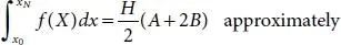
where, A = Sum of the first and last ordinates
(1.22)

B = Sum of the remaining Ordinates as Trapezoidal rule
(1.23)

1.3.1 Brownian Motion
This segment provides information for the simple solution of a Brownian movement B, along with some common variations in terminology which we use for some purposes [14]. The essential definition of B, as a random continuous function with a particular family of finite-dimensional distributions, is motivated in the appearance of this technique as a limit in distribution of rescaled random walk paths. Let (Ω, F, P) be a probability range [13].
A stochastic technique (B (T, ω), T ≥0, ω ∈Ω) is a
Brownian movement If,
1 (i) For stable each T, the random variable BT = B(T) has Gaussian distribution.
2 (ii) The procedure B has stationary independent increments.
3 (iii) For each fixed ω∈Ω, the path T→ B (T, ω) is continuous.
The which means of second point is that if, 0 ≤ T 1≤ T 2≤ T 3≤……≤ Tn then
(1.24)

are independent, and the distribution of Bti — B ti–1depends only on Ti − T i−1. According to (i), this distribution is normal with mean 0 and variance Ti − T i−1. The real B is continuous to demonstrate that B has continuous paths as in (iii). Due to the convolution properties of ordinary distributions, the joint distribution of x T1舰舰舰 xTn are predictable for any T 1≤……≤ Tn .
1.4 Results
The Numerical Example is shown in Table 1.3.
To demonstrate the solution manner introduced above, consider an Inventory object with the subsequent associated parameters ( Y ∗, T 0, N , LE , TCU(Y) , LE d ) tabulated in Table 1.4to Table 1.8.
It is presented in Table 1.9. Table 1.9is presented in Figure 1.3by using MATLAB. This model analyses how Inventory model can help in minimising the Total cost of Inventory.
The Reorder is a diffusion of enterprise. It is a price-saving technique that can assist prevent Inventory outs overlooked possibilities in business and a probable interruption in the operational technique.
The whole life pattern of a request from the maximum amount element of offer to select and decide to transportation to client conveyance.
The time it takes a Supplier to convey products after a request is set alongside the time period for a business reordering needs.
The Order Quantity is the best measure of an item to buy at a given time. It is a significant count since holding a lot of Stock is costly.
Reorder element is an approach to choose to decide when to arrange. It does not address how s extraordinary arrangement to arrange when a request is made.
Table 1.3 Optimal results of the Inventory in Various Parameters
| Parameters | Y ∗ |  |
N | LE | TCU(Y) | LEd | |
|---|---|---|---|---|---|---|---|
| 1 | k 1= $105 H=$.06 d=29 L=29 | 318.59 | 10.99 | 2.64 | -0.02 | 19.12 | -0.6 |
| 2 | k 2= $52 H=$.04 d=20 L=29 | 228.04 | 7.9 | 3.67 | 0.007 | 9.12 | 0.20 |
| 3 | k 3= $98 H=$.02 d=41 L=30 | 633.88 | 15.46 | 1.88 | -0.06 | 12.81 | -2.46 |
| 4 | k 5= $104 H=$.03 d=22 L=29 | 372.38 | 16.93 | 1.71 | 0.05 | 11.73 | 1.1 |
Table 1.4 Optimum results of the ordering processes.
 |
||||
|---|---|---|---|---|
| x | 0 | 1 | 2 | 3 |
| f(x) | 10.99 | 7.9 | 15.46 | 16.93 |
Table 1.5Optimum results of the number of integer cycles.
| N | ||||
|---|---|---|---|---|
| x | 0 | 1 | 2 | 3 |
| f(x) | 2.60 | 3.66 | 1.34 | 1.9 |
Table 1.6Optimum results of the effective lead time.
| LE | ||||
|---|---|---|---|---|
| x | 0 | 1 | 2 | 3 |
| f(x) | -0.03 | -0.012 | 0.04 | -0.039 |
Table 1.7Optimal solution of the TCU(Y).
| TCU(y) | ||||
|---|---|---|---|---|
| x | 0 | 1 | 2 | 3 |
| f(x) | 17.32 | 12.25 | 49.19 | 69.57 |
Table 1.8 Optimum results of the reorder in Le D .
| Le D | ||||
|---|---|---|---|---|
| x | 0 | 1 | 2 | 3 |
| f(x) | -0.9 | -0.36 | 1.6 | -0.78 |
Table 1.9 The optimal results of the inventory in trapezoidal rule.
| Parameters | T*0 | N | LE | TCU(y) | Le d |
|---|---|---|---|---|---|
| x | 0 | 1 | 2 | 3 | 4 |
 |
37.32 | 7.73 | -0.038 | 37.36 | -2.01 |
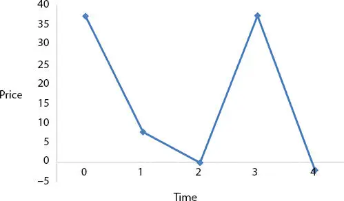
Figure 1.3 Trapezoidal rule in brownian movement.
Интервал:
Закладка:
Похожие книги на «Mathematics in Computational Science and Engineering»
Представляем Вашему вниманию похожие книги на «Mathematics in Computational Science and Engineering» списком для выбора. Мы отобрали схожую по названию и смыслу литературу в надежде предоставить читателям больше вариантов отыскать новые, интересные, ещё непрочитанные произведения.


Обсуждение, отзывы о книге «Mathematics in Computational Science and Engineering» и просто собственные мнения читателей. Оставьте ваши комментарии, напишите, что Вы думаете о произведении, его смысле или главных героях. Укажите что конкретно понравилось, а что нет, и почему Вы так считаете.