Mathematics in Computational Science and Engineering

Figure 1.2 Graphical representation of Inventory Instantaneous demand in Brownian movement.

EOQ model intent to resolve ideal number of units to arrange, so that administration can minimize the total cost associated with the purchase expense, transportation price and storage of a product. In other words, the classic EOQ is the amount of inventory to be requested per time for limiting yearly stock cost. EOQ which is profoundly act as a gadget for Inventory Control.

The proposed model is established by the following presumptions.

The Demand cost for the years is known and resupplied momentarily.

Ordering cost straight forwardly.

Inventory when an order shows up.

The management ordering cost per unit time in dollars.

Cost of ordering is stable.

Lead time for the Inventory cycle.

The Lead time, that is the time between the putting of the request and the receiving of the order is known.

There is no restraint on order size.

An order is a request for something to be provided.

Ordering costs which may be caused an acquiring extra Inventories. The more regularly arranges are put and less the amounts bought on each request.

There is no quantity concession.

To survey the hidden suspicions of the EOQ model for the improved apprehension of current Inventory Management.

Shortages are not permitted.

The accompanying documentation is utilized to build up the model.

d = Total number of units produced.

k 1= Set up cost related to the arrangement of orders. L = additionally appear some of the region Q = Order quantity. Ic = The Stock processes for this pattern is time units. Y ∗ = Order the Quantity in every day. N = the number of highest integers. H = Holding cost per unit every day. S = No Shortage is allowed. R = Reorder point. LEd = The reorder point accordingly happens when the Inventory level drops. A = Sum of the initial and end ordinates. B = Sum of the final Ordinates as Trapezoidal rule. C = Item Cost

The mathematical method confesses the Inventories position and it is expressed as

Thing is also diminished at the ordinary demand amount d.

The ordering period for the models is

Put that the Normal Inventory stage is

The total price per unit time (TCU) is along these lines figured out as TCU(y) = Set up cost per unit time + Holding Cost per unit time

(1.14)

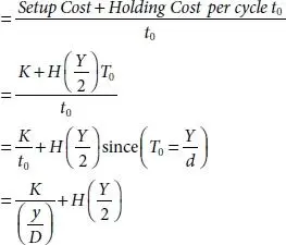
The most helpful assessment putting in a request sum y is controlled with method of reduce TCU(y) concerning y. Consider y is fundamental circumstance for finding the ideal assessment of y.

Here Y assumed as continuous,

(1.15)

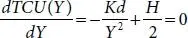
The terms are additionally sufficient because of the reality TCU(y) is Convex.

The result of the situation yields the EOQ, y*as

Subsequently the most ideal Inventory strategy for the propounded model is

(1.16)

Units every time.

A new order needs no longer be acquired in the meanwhile it is ordered. Rather than of high-quality Lead time L, may also additionally appear some of the region and the receipt of an order as Reorder element inside the exemplary EOQ models. In this situation the reorder aspect shows up even as the Inventory degree drops to LD units.

Reorder point inside the conventional EOQ version assumes that the lead time L is an awful lot much less than the cycle period which may not be the case in extensively well known. Lead time that is the quantity of time among placing an order and accepting the stock.

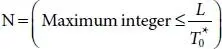
Effective lead time is defined as

(1.17)

where n is the highest integer not exceeding

The range of integer cycle consists of in L is

(1.18)

Each the Inventory situation acts as if the interval amongst setting an order and getting another is Le .

The reorder factor as a result takes area while the Inventory degree drops to Le D .

This research became applied quantitative research design to measured data due to Numerical and to get appropriate and specific statistics the frame of the researchers. This model examines how Inventory model can assist in minimising the total cost of Inventory model. The Trapezoidal guideline works by approximating the region under the graph of the capacity f(x) as Trapezoid and computing its area. It is ruled to locate the estimation of a positive fundamental utilizing numerical technique.

(1.19)