Mathematics in Computational Science and Engineering

It became accepted that there might be no time along requesting and buying of materials. The ascertaining Reorder level includes the figuring of utilization cost every day. Consider an association that works with a provider. The organization stores a few items renew by the providers to fulfil its Customers need.

Figure 1.3. Depicts the applicable of Inventories of Parameters Y ∗, T 0 , N, LE , TCU(Y) , Le d calculation and the subsequent optimization of Inventories with the aim of minimizing the proposed goal.

This Numerical Example to illustrate the above Mathematical model.

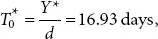
Parameters 1 : k 1= $105, H = $.06, d = 29 units per day L = 29 days. Optimal solutions Y* = 346.41, 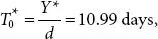N = 2.64, L E = −0.02days, LeD = −0.6, The everyday Inventory price related with the Expected Inventory scheme is TCU(y) = 19.12.

Parameters 2 : k 1= $52, H = $.04, d = 20 units per day L = 29 days. Optimal solutions Y* = 228.04, 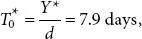N= 3.67, LE = 0.007 days, LeD = 0.203., The everyday Inventory price related with the Expected Inventory scheme is TCU(y) = 9.12.

Parameters 3 : k 1= $98, H = $.02, d = 41 units per day L = 29 days. Optimal solutions Y* = 633.88, 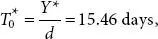N = 1.88, LE = −0.06 days, LeD = −2.46, The everyday Inventory price related with the Expected Inventory scheme is TCU(y) = 12.81.

Parameters 4 : k 1= $104, H = $.03, d=22 units per day L = 29 days. Optimal solutions Y* = 372.38, N = 1.71, LE = 0.05 days, LeD = 1.1, The everyday Inventory price related with the Expected Inventory scheme is TCU(Y) = 11.73.

The EOQ model of Inventory Management takes over the day-by-day utilization of Inventories, the optimum estimation of the orders amount y is controlled by minimizing TCU(Y).

The study effects of change in the value of the system are displayed from Table 1.4to Table 1.9. This is

Important Inventory Parameters ( Y ∗, T 0, N , LE , TCU(Y) , LEd ) are classified.

By Parameters 1: The set-up cost increases, diminishes, n decreases, LE decreases and LEd decrease, then The Everyday Inventory expense joined with the propounded Inventory scheme is TCU(y) diminishes.

By Parameters 2: The set-up cost increases, decreases, N decreases, LE Decreases and LEd decrease, then The Everyday Inventory expense joined with the propounded Inventory plot is TCU(Y) diminishes.

By Parameters 3: The set-up expense increases, decreases, N diminishes, LE Decreases and LEd decrease, The Everyday Inventory Cost combined with the propounded Inventory scheme is TCU(Y) diminishes.

By Parameters 4: The set-up cost expands, diminishes, N diminishes, LE Decreases and LEd decreases, The Everyday Inventory price joined with the propounded Inventory scheme is TCU(Y) Increases.

This Y* is not Trapezoidal Rule and hence it is not formed a Brownian movement, but remaining Parameters T 0, N , LE, LEd , TCU(Y) is a Trapezoidal Rule. It is framed a Brownian Movement.

At last implementing Sensitivity assessment on the decision factors through changing the Inventory parameters ( Y ∗, T 0, N, LE, LEd , TCU(Y). In sensitivity investigation make fluctuate to the factors built into that Inventory to provide the Brownian movement. This method is generally sensitivity to change around the EOQ.

Brownian direction is a-Holder a. s. for all A Brownian movement is sort of really now not -Holder. However, there does represent a t = t ( w ) such that

(1.25)

For every h most definitely. The decided of such t offer degree zero. This is the moderate improvement that is locally possible. Having confirmed that Brownian direction are extremely popular [19]. Make see why they are “peculiar”. One rationalization is that the strategies of Brownian movement don’t get any time of monotonicity. Indeed, if [a,b] is an time of monotonicity, at that point splitting it into an equivalent sub-period [ ai, a i+1] every expansion B ( ai ) – B ( a i+1) should have a similar indication. This has probability 2.2 −nand taking n→ ∞ indicates that the probability that [ a, b ] is a time of monotonicity ought to be [13]. Let a countable association prove that there may be no gap of monotonicity with rational that Brownian movement solution, however each monotone. Period could have a monotone logical alternate period that Brownian movement is b -Holder for any a.S. This will infer us to conclude a higher certain on the Hausdorff measurement of the graph [12]. Reproduce that the graph Gf of a feature f is the fix of factors (t, f (t)) as t degrees over the area off. it will permit us to infer a top positive at the Hausdorff length of the graph [12]. Review outlines Gf of an event f is the fix of things (t, f (t)) as t levels outer the area of f.

The Hausdorff degree of a self-affine set ought be either 0 or ∞. Assume the number set d has non-uniform parallel fibers and let γ = dim (K (d), then H γ( K ( d )) = ∞.