Mathematics in Computational Science and Engineering
Здесь есть возможность читать онлайн «Mathematics in Computational Science and Engineering» — ознакомительный отрывок электронной книги совершенно бесплатно, а после прочтения отрывка купить полную версию. В некоторых случаях можно слушать аудио, скачать через торрент в формате fb2 и присутствует краткое содержание. Жанр: unrecognised, на английском языке. Описание произведения, (предисловие) а так же отзывы посетителей доступны на портале библиотеки ЛибКат.
- Название:Mathematics in Computational Science and Engineering
- Автор:
- Жанр:
- Год:неизвестен
- ISBN:нет данных
- Рейтинг книги:4 / 5. Голосов: 1
-
Избранное:Добавить в избранное
- Отзывы:
-
Ваша оценка:
Mathematics in Computational Science and Engineering: краткое содержание, описание и аннотация
Предлагаем к чтению аннотацию, описание, краткое содержание или предисловие (зависит от того, что написал сам автор книги «Mathematics in Computational Science and Engineering»). Если вы не нашли необходимую информацию о книге — напишите в комментариях, мы постараемся отыскать её.
This groundbreaking new volume, written by industry experts, is a must-have for engineers, scientists, and students across all engineering disciplines working in mathematics and computational science who want to stay abreast with the most current and provocative new trends in the industry.
This groundbreaking new volume: Includes detailed theory with illustrations Uses an algorithmic approach for a unique learning experience Presents a brief summary consisting of concepts and formulae Is pedagogically designed to make learning highly effective and productive Is comprised of peer-reviewed articles written by leading scholars, researchers and professors AUDIENCE:
Mathematics in Computational Science and Engineering — читать онлайн ознакомительный отрывок
Ниже представлен текст книги, разбитый по страницам. Система сохранения места последней прочитанной страницы, позволяет с удобством читать онлайн бесплатно книгу «Mathematics in Computational Science and Engineering», без необходимости каждый раз заново искать на чём Вы остановились. Поставьте закладку, и сможете в любой момент перейти на страницу, на которой закончили чтение.
Интервал:
Закладка:
The numerical created model for resulting documentation and assumptions.
1.2.3.1 Assumptions
The accompanying assumptions are considered to build up this model.
The request cost for the thing is Inventory organized.
Shortages are allowed.
Instantaneous request and stable Replenishment.
Stock decayed during the arranging skyline are repairable.
Holding cost, Set-up cost, Shortage cost and unit cost stay consistent over the long run.
The dispersion of an opportunity to fall apart follows a four Parameters.
Replenishment is quick.
1.2.3.2 Notations
This section begins with a listing of the Notations used.
S = Highest Stock stage.
f (d) = Probability density characteristic of Demand.
D = Deterioration.
Q = Optimum production order amount.
CS = Shortage price. CH = Holding Price per unit per unit of duration held in Stock. Q* = Back ordering is permitted. I = units per year C = Unit price for producing or purchasing every unit, TEC 1(Q) = Optimum Inventory achieve local minimum. TEC 1(I)= Expected price. TEC (Q*) = Conditional for Ordering.
1.2.3.3 Model Formulation
This model is the same as fixed setup cost for buying any units to renew Stock at start of period, say K, is related buy or making things in a given timeframe or cost of assembling. Leave I alone the Inventory stage toward the start of the level infers that a request size (Q-I) thing can be set to pass on the available Inventory up to Q. Hence, the anticipated cost transforms into,
(1.7) 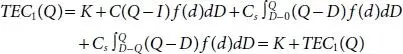
The optimal value of Q says Q* that minimizes TEC 1(Q)) is given by
(1.8) 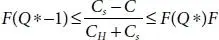
where
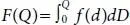
Since K is constant, minimum value of TEC’ (Q) ought to additionally accept via the same condition as given in equation
(1.9) 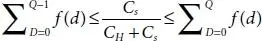
Since K is constant, minimum value of
And consequently Q* can even decrease TEC (Q).
Let us present two new control factors S and s, where S represents the extreme Stock stage and s signifies the reordered stage that is while the Stock degree tumbles to s, a request is situated to bring the Stock of Inventory items up to S.
Thus, value of S= Q* and the price of s is determined by the relationship
(1.10) 
As I the fundamental Inventory prior to starting the period, at that point to decide the request size to bring the available Inventory of articles as much as Q*, the ensuing three occasions might be examined.

Case 1: If we start the length with I unit of Inventory and do not now buy or produce more prominent, at that point TEC (I) is the foreseen cost. In any case, on the off chance that we expect to purchase extra (Q-I) units in the event that you need to convey Inventory stage as much as Q*, at that point TEC’ (Q*) will include the set-up expense furthermore. Subsequently, for all I
(1.11) 
That is, while Inventory stage arrives at S=Q*, request for Q-I units of Inventory might be put.
Case 2: For this situation, if I
(1.12)
This implies that no ordering substantially less costly than ordering. Thus Q*=I.
Case 3: If Q>I, at that point foreseen cost for a request up to Q could be extra than generally speaking foreseen cost if no structure is found, that is
(1.13)
Consequently, it is better not to put request for acquirement of things and afterward Q*=I.
1.2.3.4 Numerical Examples
In framework to exhibit the proposed model, a Numerical model is settled with the accompanying Parameters value I=10, CH =0.53, Cs=Rs 5, C=2.5 and K=25. At that point get ideal arrangements are Q*= 45, TEC 1(I)=202.79, TEC 1(Q)=168.5, TEC (Q*) =193.5. Figured outcomes are demonstrated in Table 1.2.
Table 1.2 Optimal instantaneous demand solution of the order policy.
| Parameters | Q* | TEC1 (I) | TEC1 (Q) | (TEC (Q *) |
|---|---|---|---|---|
| I=10, CH = 0.53 CS = Rs 5 ,C = 2.5 andK 1 = 25 | 45 | 202.79 | 168.5 | 193.5 |
| I=10, CH = 0.54 CS = Rs 7 ,C = 3.5 andK 2 = 26.5 | 46 | 283.77 | 233.77 | 260.27 |
| I=10, CH = 0.51 CS = Rs 8.5 ,C = 4.5 andK 3 = 27.5 | 44 | 344.51 | 291.22 | 318.72 |
| I=10, CH = 0.52 CS = Rs 9.5 ,C = 5.5 andK 4 = 28.5 | 40 | 385.01 | 340.16 | 368.66 |
| I=10, CH = 0.52 CS = Rs 10.5 ,C = 6.5 andK 5 = 29.5 | 36 | 425.51 | 387.41 | 416.91 |
1.2.3.5 Sensitivity Analysis
Sensitivity analysis is performed in this section with respect to crucial parameter. We change the value parameter by Q*, TEC 1(I), TEC 1(Q), TEC (Q*) individually keeping different boundaries at their unique qualities and noticed its impact on ideal approach. This demonstrates that as the Ordered quantity increases (Q*), Expected cost Increases TEC(I), Optimum Stock achieve local minimum TEC(Q) decreases, Condition for Ordering TEC (Q*) is increments. Thus, the Sensitivity of the ideal outcome to little change in the Parameter esteem is inspected. Legitimate Inventory limit the Ordering cost of the multiplying. Proposed model be thing by taking various suppositions cost of Inventory value Parameters. The outcomes are presented in Table 1.2. Table 1.2is displayed in Figure 1.2.
Интервал:
Закладка:
Похожие книги на «Mathematics in Computational Science and Engineering»
Представляем Вашему вниманию похожие книги на «Mathematics in Computational Science and Engineering» списком для выбора. Мы отобрали схожую по названию и смыслу литературу в надежде предоставить читателям больше вариантов отыскать новые, интересные, ещё непрочитанные произведения.


Обсуждение, отзывы о книге «Mathematics in Computational Science and Engineering» и просто собственные мнения читателей. Оставьте ваши комментарии, напишите, что Вы думаете о произведении, его смысле или главных героях. Укажите что конкретно понравилось, а что нет, и почему Вы так считаете.